[!] Class technology
Technology in the model represents a type of process that convert one (or several) type of commodity to another (or several others). Function newTechnology() creates a technology object.
ATECH <- newTechnology("ATECH")
slotNames(ATECH)
## [1] "name" "description" "input"
## [4] "output" "aux" "units"
## [7] "group" "cap2act" "geff"
## [10] "ceff" "aeff" "af"
## [13] "afs" "weather" "fixom"
## [16] "varom" "invcost" "start"
## [19] "end" "olife" "stock"
## [22] "early.retirement" "upgrade.technology" "fullYear"
## [25] "slice" "region" "misc"
## [28] ".S3Class"This class has more comprehensive set of parameters vs others with a goal to be able to model a broad range of technological processes. Therefore technology has 28 slots.
show structure
str(ATECH)## Formal class 'technology' [package "energyRt"] with 28 slots
## ..@ name : chr "ATECH"
## ..@ description : chr ""
## ..@ input :'data.frame': 0 obs. of 4 variables:
## .. ..$ comm : chr(0)
## .. ..$ unit : chr(0)
## .. ..$ group : chr(0)
## .. ..$ combustion: num(0)
## ..@ output :'data.frame': 0 obs. of 3 variables:
## .. ..$ comm : chr(0)
## .. ..$ unit : chr(0)
## .. ..$ group: chr(0)
## ..@ aux :'data.frame': 0 obs. of 2 variables:
## .. ..$ acomm: chr(0)
## .. ..$ unit : chr(0)
## ..@ units :'data.frame': 0 obs. of 4 variables:
## .. ..$ capacity: chr(0)
## .. ..$ use : chr(0)
## .. ..$ activity: chr(0)
## .. ..$ costs : chr(0)
## ..@ group :'data.frame': 0 obs. of 3 variables:
## .. ..$ group : chr(0)
## .. ..$ description: chr(0)
## .. ..$ unit : chr(0)
## ..@ cap2act : num 1
## ..@ geff :'data.frame': 0 obs. of 5 variables:
## .. ..$ region : chr(0)
## .. ..$ year : int(0)
## .. ..$ slice : chr(0)
## .. ..$ group : chr(0)
## .. ..$ ginp2use: num(0)
## ..@ ceff :'data.frame': 0 obs. of 14 variables:
## .. ..$ region : chr(0)
## .. ..$ year : int(0)
## .. ..$ slice : chr(0)
## .. ..$ comm : chr(0)
## .. ..$ cinp2use : num(0)
## .. ..$ use2cact : num(0)
## .. ..$ cact2cout: num(0)
## .. ..$ cinp2ginp: num(0)
## .. ..$ share.lo : num(0)
## .. ..$ share.up : num(0)
## .. ..$ share.fx : num(0)
## .. ..$ afc.lo : num(0)
## .. ..$ afc.up : num(0)
## .. ..$ afc.fx : num(0)
## ..@ aeff :'data.frame': 0 obs. of 21 variables:
## .. ..$ acomm : chr(0)
## .. ..$ comm : chr(0)
## .. ..$ region : chr(0)
## .. ..$ year : int(0)
## .. ..$ slice : chr(0)
## .. ..$ cinp2ainp: num(0)
## .. ..$ cinp2aout: num(0)
## .. ..$ cout2ainp: num(0)
## .. ..$ cout2aout: num(0)
## .. ..$ act2ainp : num(0)
## .. ..$ act2aout : num(0)
## .. ..$ cap2ainp : num(0)
## .. ..$ cap2aout : num(0)
## .. ..$ ncap2ainp: num(0)
## .. ..$ ncap2aout: num(0)
## .. ..$ stg2ainp : num(0)
## .. ..$ sinp2ainp: num(0)
## .. ..$ sout2ainp: num(0)
## .. ..$ stg2aout : num(0)
## .. ..$ sinp2aout: num(0)
## .. ..$ sout2aout: num(0)
## ..@ af :'data.frame': 0 obs. of 8 variables:
## .. ..$ region : chr(0)
## .. ..$ year : int(0)
## .. ..$ slice : chr(0)
## .. ..$ af.lo : num(0)
## .. ..$ af.up : num(0)
## .. ..$ af.fx : num(0)
## .. ..$ rampup : num(0)
## .. ..$ rampdown: num(0)
## ..@ afs :'data.frame': 0 obs. of 6 variables:
## .. ..$ region: chr(0)
## .. ..$ year : int(0)
## .. ..$ slice : chr(0)
## .. ..$ afs.lo: num(0)
## .. ..$ afs.up: num(0)
## .. ..$ afs.fx: num(0)
## ..@ weather :'data.frame': 0 obs. of 11 variables:
## .. ..$ weather: chr(0)
## .. ..$ comm : chr(0)
## .. ..$ wafc.lo: num(0)
## .. ..$ wafc.up: num(0)
## .. ..$ wafc.fx: num(0)
## .. ..$ waf.lo : num(0)
## .. ..$ waf.up : num(0)
## .. ..$ waf.fx : num(0)
## .. ..$ wafs.lo: num(0)
## .. ..$ wafs.up: num(0)
## .. ..$ wafs.fx: num(0)
## ..@ fixom :'data.frame': 0 obs. of 3 variables:
## .. ..$ region: chr(0)
## .. ..$ year : int(0)
## .. ..$ fixom : num(0)
## ..@ varom :'data.frame': 0 obs. of 8 variables:
## .. ..$ region: chr(0)
## .. ..$ year : int(0)
## .. ..$ slice : chr(0)
## .. ..$ comm : chr(0)
## .. ..$ acomm : chr(0)
## .. ..$ varom : num(0)
## .. ..$ cvarom: num(0)
## .. ..$ avarom: num(0)
## ..@ invcost :'data.frame': 0 obs. of 3 variables:
## .. ..$ region : chr(0)
## .. ..$ year : int(0)
## .. ..$ invcost: num(0)
## ..@ start :'data.frame': 0 obs. of 2 variables:
## .. ..$ region: chr(0)
## .. ..$ start : num(0)
## ..@ end :'data.frame': 0 obs. of 2 variables:
## .. ..$ region: chr(0)
## .. ..$ end : num(0)
## ..@ olife :'data.frame': 0 obs. of 2 variables:
## .. ..$ region: chr(0)
## .. ..$ olife : num(0)
## ..@ stock :'data.frame': 0 obs. of 3 variables:
## .. ..$ region: chr(0)
## .. ..$ year : int(0)
## .. ..$ stock : num(0)
## ..@ early.retirement : logi TRUE
## ..@ upgrade.technology: chr(0)
## ..@ fullYear : logi TRUE
## ..@ slice : chr(0)
## ..@ region : chr(0)
## ..@ misc : list()
## ..@ .S3Class : chr "technology"The key concepts in technology are:
- capacity;
- two levels of activity (use and activity);
- core input and output commodities, which form the activity of the technological process;
- auxiliary input and output commodities, which depend on the core variables;
- (a chain of) efficiency parameters to transform one core commodity or activity to another;
- auxiliary efficiency parameters to link auxiliary commodities to core variables;
Core input and output
The minimal set of parameters to declare technology includes its name, input and output commodities. draw() method sketches the structure of the technology.
ATECH <- newTechnology(
name = "ATECH",
description = "A technology",
input = list(
comm = "CINP",
unit = "UnitInp"
),
output = list(
comm = "COUT",
unit = "UnitOut"
)
)
draw(ATECH)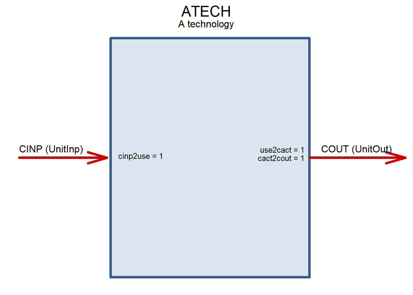 Arrows on the sketch describe commodities flow.
Capacity and Activity
Every technology is characterized by its maximum instant (or nameplate) capacity to produce a commodity(-ies), and its activity in time. capacity is a technological resource, while activity is a usage of the resource. Both can be partially or entirely exogenous or endogenous, meaning their level is defined on the stage of the model formulation by a modeler, or can be a result of the optimization - the model solution.
It is important to identify the main activity commodity of the technology and set units of activity and capacityfor every technology. The relation between capacity and activity units is set by parameter cap2act in the slot @cap2act. The default value of the parameter is equal to 1, meaning that capacity of the technology is measured in annual units, for example in million tones of steel a year.
ATECH@cap2act## [1] 1Alternatively, if the technology is a coal power plant with the main electricity (ELC) as the main commodity output, the capacity is normally measured in watts, megawatts or gigawatts. The activity commodity can be simply measured in the main commodity units. Therefore, if electricity in the model is measured in gigawatt hours (“GWh”) and capacity in gigawatts (“GW”) then cap2act is simply a number of hours in the year: cap2act = 8760.
ECOA <- newTechnology(
  name = "ECOA",
  description = "Coal-fired power plant",
  input = list(
    comm = "COA",
    unit = "PJ"
  ),
  output = list(
    comm = "ELC",
    unit = "GWh"
  ),
  cap2act = 24 * 365
)
ECOA@cap2act
## [1] 8760However, if all energy commodities in the model, including ELC are measured in petajoules (“PJ”) then capacity variable and commodity output variable have different units and should be adjusted. There are several ways to do that in the model. First, and the simplest one is to adjust cap2act to the conversion coefficient between the two units. In our case, annual output of 1 GW of installed capacity can produce up to 8760 GWh, that is an equivalent of 31.536 PJ.
ECOA <- update(ECOA,
               cap2act = 24 * 365 * convert(from = "GWh", to = "PJ"),
               output = list(comm = "ELC", unit = "PJ") # changing units from GWh
               )
ECOA@cap2act
## [1] 31.536Units or electricity in this example should be also changed to “PJ”. Or alternatively the activity of the technology can stay in “PJ” but the output can be converted using cact2cout parameter is slot @ceff as discussed later.
Multiple input and output
In most cases technological processes are more complicated and have more main inputs, outputs, or associated consumed, produces, or emitted commodities. There are groups of such parameters in energyRt to model different types of relations.
Complementary commodities (Leontief function)
If shares of all inputs or outputs are fixed and the same in every moment of production, they can be modeled as equal main commodities by adding directly to the @input and/or @output slots. Continuing our example of coal power plant, lets add biomass “BIO” co-firing in the inputs.
# Coal only
ECOA@input
## comm unit group combustion
## 1 COA PJ <NA> NA# Adding biomass (BIO)
ECOA <- update(ECOA, input = list(comm = c("COA", "BIO"),
unit = c("PJ", "PJ")))
ECOA@input## comm unit group combustion
## 1 COA PJ <NA> NA
## 2 BIO PJ <NA> NAdraw(ECOA)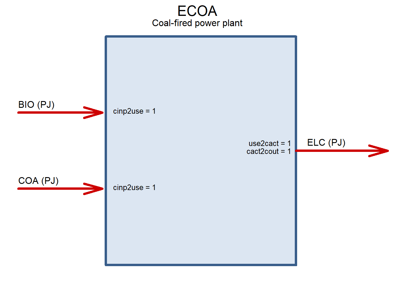 In this example both commodities “COA” and “BIO” are required to produce electricity with this technology. (Efficiency parameters are considered later)
Let’s now assume that the power plant also produces heat (“HEA”) and the ratio between two output commodity is also fixed. To declare HEA as an additional main output it should be declared in the @output slot the same way as for input.
co-firing in the inputs.
# Electricity only
ECOA@output
## comm unit group
## 1 ELC PJ <NA># Adding heat (HEA)
ECOA <- update(ECOA, output = list(comm = c("ELC", "HEA"),
unit = c("PJ", "PJ")))
ECOA@output## comm unit group
## 1 ELC PJ <NA>
## 2 HEA PJ <NA>draw(ECOA)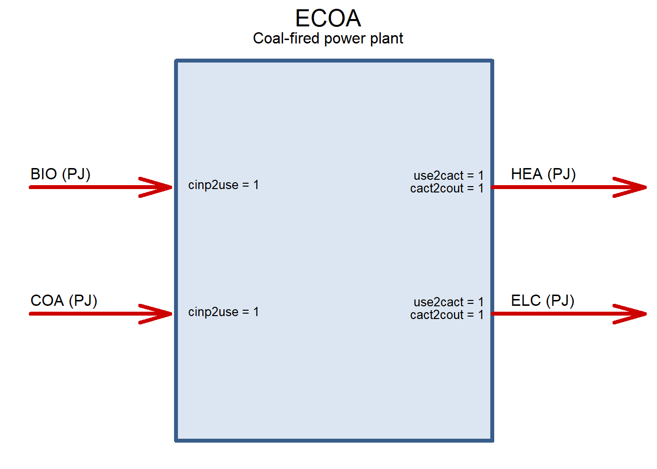 Both output commodities are declared as the main (core) commodities. Sum of their activity will be considered as the
 activity of the technology. (The required parameters will be set later)
Commodities-substitutes (Linear function)
Alternative scenario is when the two commodities can be substitutes. If “BIO” is not available (or too expensive), then “COA” can be used instead and vice versa. To declare substitution between commodities, they should be grouped by adding the same caracter name for the commodities to the group column in the same @input slot.
ECOA <- update(ECOA, input = list(comm = c("COA", "BIO"),
                                  unit = c("PJ", "PJ"),
                                  group = c("i", "i")))
ECOA@input
## comm unit group combustion
## 1 COA PJ i NA
## 2 BIO PJ i NAdraw(ECOA)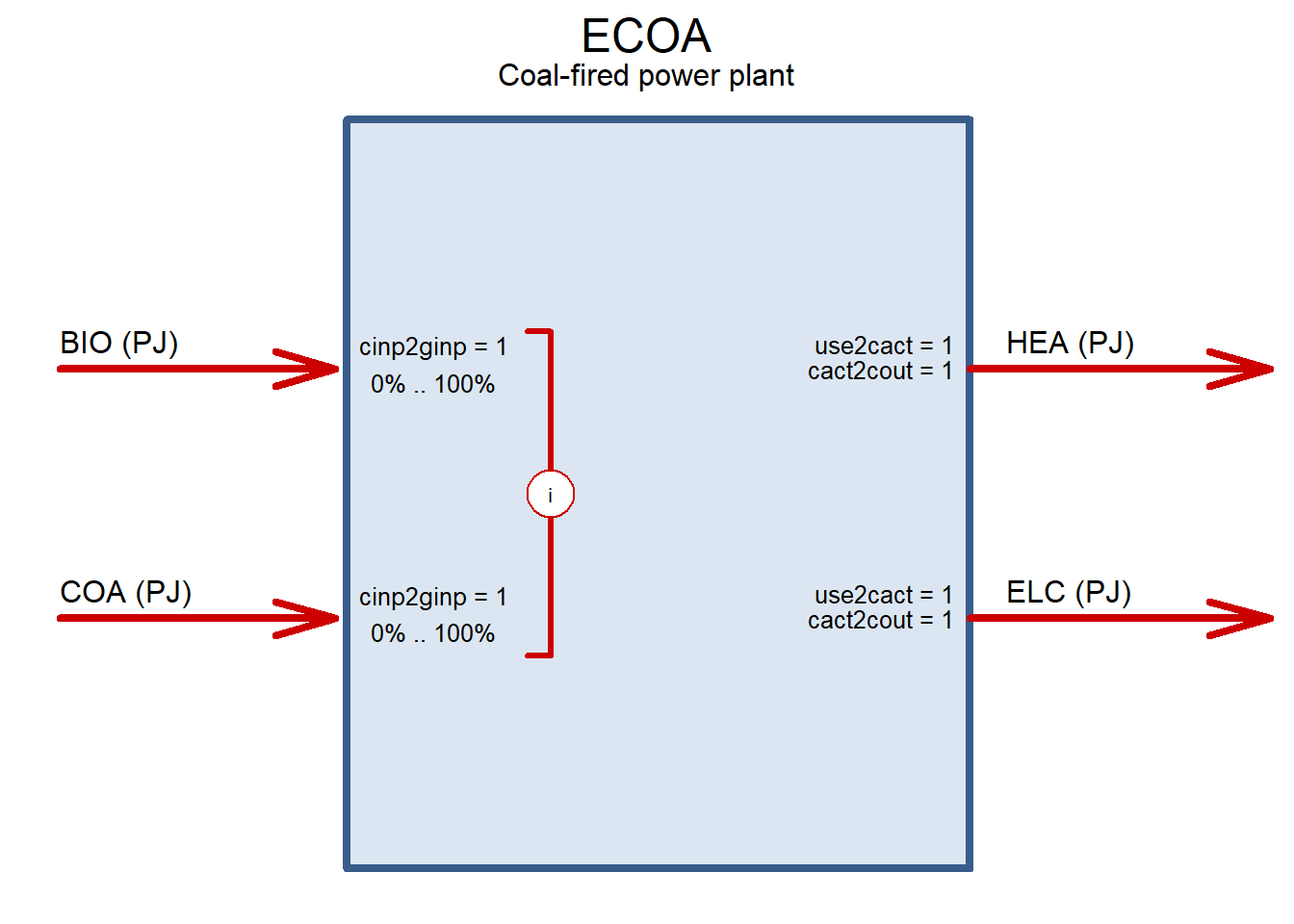 Names of groups can repeat in different technologies, they will not interfere in the model code.
Output commodities can be grouped the same way as input, by assigning a character name of the output group against output commodities in the @output slot. Let’s call the technology differently - combined heat and power plant.
ECOA@output## comm unit group
## 1 ELC PJ <NA>
## 2 HEA PJ <NA>ECHP <- update(ECOA,
description = "Coal-fired CHP plant",
output = list(comm = c("ELC", "HEA"),
unit = c("PJ", "PJ"),
group = c("o", "o")))
ECHP@output## comm unit group
## 1 ELC PJ o
## 2 HEA PJ odraw(ECHP)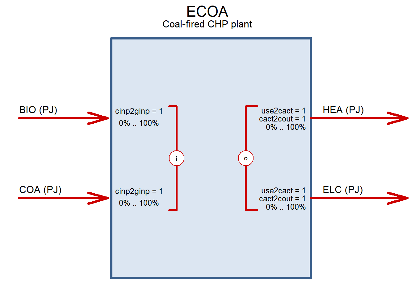 With those settings the technology can equally produce electricity and/or heat in any proportion using coal or biomass or both.
Efficiency
In the example above CHP plan had all efficiency parameters equal to their default value (= 1) meaning that efficiency of the process is equal to 100%. One unit of input (COA or BIO) will produce one unit of output (ELC or HEA). Efficiency parameters for main commodities are stored in @ceff (commodity efficiency) and @geff (group efficiency) slots.
Commodity-level efficiency
str(ECHP@ceff)## 'data.frame': 0 obs. of 14 variables:
## $ region : chr
## $ year : int
## $ slice : chr
## $ comm : chr
## $ cinp2use : num
## $ use2cact : num
## $ cact2cout: num
## $ cinp2ginp: num
## $ share.lo : num
## $ share.up : num
## $ share.fx : num
## $ afc.lo : num
## $ afc.up : num
## $ afc.fx : num