COMM <- newCommodity("COMM")
class(COMM)
[1] "commodity"
attr(,"package")
[1] "energyRt"slotNames(COMM)[1] "name" "desc" "limtype" "timeframe" "unit" "emis"
[7] "agg" "misc" energyRt/timeslices packagecommodityCommodity in the model is a broad notion of any a substance, material, energy, goods, or services that can be exchanges, produced, transformed to another commodity(-ies) by a technology or used for a final consumption in the model. Examples: electricity, coal, gas, steel, cement, CO2, CH4 etc.
COMM <- newCommodity("COMM")
class(COMM)[1] "commodity"
attr(,"package")
[1] "energyRt"slotNames(COMM)[1] "name" "desc" "limtype" "timeframe" "unit" "emis"
[7] "agg" "misc" The structure of a class can be printed with str() function.
str(COMM)Formal class 'commodity' [package "energyRt"] with 8 slots
..@ name : chr "COMM"
..@ desc : chr ""
..@ limtype : Factor w/ 3 levels "FX","UP","LO": 3
..@ timeframe: chr(0)
..@ unit : chr(0)
..@ emis :'data.frame': 0 obs. of 3 variables:
.. ..$ comm: chr(0)
.. ..$ unit: chr(0)
.. ..$ emis: num(0)
..@ agg :'data.frame': 0 obs. of 3 variables:
.. ..$ comm: chr(0)
.. ..$ unit: chr(0)
.. ..$ agg : num(0)
..@ misc : list()The commodity class has 8 slots. The first two name and desc are the same in all energyRt classes, representing the name in the model sets (commodity in this case) and optional description. Names should follow the conversions used in GAMS, Python/Pyomo, Julia/JuMP, or GLPK/MathProg, as well as R. All the languages have a little bit different conventions regarding special characters and case sensitivity. The rule of thumb is a) case sensitivity and (b) avoiding special characters including whitespace (), period (.), hyphen or dash (-).
As an example, GAMS is not case sensitive, lower and upper case letters treated are considered the same characters. However R, and all other mentioned above mathematical languages use distinct (case-sensitive) names for sets, parameters, and variables. To avoid potential inconsistencies and bugs, it is recommended to use all names of the model elements in the same upper or lower case. Here in the manual we use upper case letters for all short names, used in the model sets, and avoid all special characters except underscore (_).
Commodities are not region-specific. They must be declared only once for all regions in the model. Though their appearance in different regions will depend on available processes (see Class supply section).
The net quantity (balance) of every commodity in the model is constrained by lower (LO or UP FX LO meaning that the total net quantity of the commodity in the model must be equal or higher than the total amount of all intermediate and final demands, as indicated by equations ___. Changing the default value can be done using the limtype parameter in the newCommodity or update functions:
COMM@limtype[1] LO
Levels: FX UP LOCOMM <- newCommodity("COMM", desc = "Some commodity", limtype = "FX")
COMM@limtype[1] LO
Levels: FX UP LOor
COMM <- update(COMM, limtype = "UP")
COMM@limtype
[1] UP
Levels: FX UP LOA direct assignment is also possible but not recommended to avoid potential mismatches between data types or allowed values. This type of direct assignment COMM@limtype <- "LO" will not work because class factor is expected as an input:
class(COMM@limtype)[1] "factor"A proper way would be to create a factor with expected values and assign it:
COMM@limtype <- factor("LO", levels = c("FX", "UP", "LO"))
COMM@limtype
[1] LO
Levels: FX UP LOHowever this process is more complicated and sensitive to potential changes in the package. Function newCommodity and method update will do the job. It is a generic recommendation to use such helper functions for assigning or updating values in all S4 classes.
Depending on the model purpose, commodities can have different level of sub-annual granularity. For example, in an hourly model with 8760 sub-annual time slices (24 hours * 365 days) a balance between production and consumption of electricity should hold for every hour. However, it makes less sense to track other commodities, such as coal or natural gas, by hours. It might be enough if their balances can be hold on daily or even annual basis. This will significantly reduce dimensionality of the model without sacrificing any important for the study details.
ELC <- newCommodity("ELC", desc = "Electricity", timeframe = "HOUR")
GAS <- newCommodity("GAS", desc = "Natural gas", timeframe = "YDAY")
COA <- newCommodity("COA", desc = "Hard coal", timeframe = "ANNUAL")
In this example generation and consumption of electricity (ELC) will be modeled for every hour of the model (8760 per year), natural gas (GAS) equations will have daily equations (365 per year), and coal (COA) will have no sub-annual resolution (1 per year). The default value of the slice is the lowest level of time-slices in the model. In this example, the lowest level will be “HOUR”. It will be assigned to all commodities by default if it is not set explicitly.
All commodities are normally measured and tracked in physical units such as Jules, watt-hours, kg or million tonnes, etc. This slot (@unit) is currently used for information only to document units of the data used in the model. They will play an important role in estimation of the efficiency parameters and costs in other classes of the model.
ELC <- newCommodity("ELC", desc = "Electricity", timeframe = "HOUR", unit = "GWh")
GAS <- newCommodity("GAS", desc = "Natural gas", timeframe = "YDAY", unit = "PJ")
IRON <- newCommodity("IRON", desc = "Iron metal", timeframe = "ANNUAL", unit = "kt")In some cases it is handy from modeling perspectives to aggregate several commodities into one that can be further used for modeling policy or any other purposes. For example, there is a broad range of different type of greenhouse gases (GHG), such us carbon dioxide (CO2), methane (CH4), Nitrous oxide (N2O). From a policy perspective and for modeling purposes it might be helpful to combine all of them together into one GHG ‘commodity’ using global warming potential weights (100 years in this example). 1
# Create different GHG commodities
CO2 <- newCommodity("CO2", desc = "Carbon dioxide", unit = "kt")
CH4 <- newCommodity("CH4", desc = "Methane", unit = "kt")
N2O <- newCommodity("CO2", desc = "Nitrous oxide", unit = "kt")
# Now aggregate them into one
GHG <- newCommodity("GHG", desc = "Greenhouse gases", unit = "kt",
                    agg = data.frame(
                      comm = c("CO2", "CH4", "CO2"),
                      unit = rep("kt", 3),
                      agg = c(1, 30, 273)
                    ))
The data.frame assigns aggregating (agg) values to each of the commodities. In the model such aggregating commodities will co-exist with the aggregated components as an additional measurement indicator. It can be consumed or produced by other processes the same way as other commodities.
GHG@agg comm unit agg
1 CO2 kt 1
2 CH4 kt 30
3 CO2 kt 273supplyThere are three ways for a commodity to appear in the model, through supply, import, or as an output of a modeled process. (An exception is an aggregating commodity, though its components still take at least one of the three ways to appear in the model.)
Class supply describes the market of a commodity that can be acquired in a certain volume at a certain price. If the process of production of a commodity is beyond the focus of the study, it can be modeled via supply or import. The only difference between the two is that supply is considered as a domestic resource, while import - as an external to the modeled regions. Supply is an exogenous resource for consideration in the optimization process. It can have different features, can be exhaustible or infinite, have different shapes and costs by time-slices, years, or regions. A new supply or resource cannot be created during the optimization process, available resources with predefined features are 100% exogenous to the model.
Function newSupply creates an object of class supply similarly to the class commodity. The example below creates supply of coal in the model.
SUPCOA <- newSupply(name = "SUPCOA",
                    desc = "Supply of coal",
                    commodity = "COA",
                    unit = "PJ")
class(SUPCOA)
[1] "supply"
attr(,"package")
[1] "energyRt"slotNames(SUPCOA)[1] "name" "desc" "commodity" "unit" "weather"
[6] "reserve" "availability" "region" "misc" Class supply has 9 slots.
str(SUPCOA)Formal class 'supply' [package "energyRt"] with 9 slots
..@ name : chr "SUPCOA"
..@ desc : chr "Supply of coal"
..@ commodity : chr "COA"
..@ unit : chr "PJ"
..@ weather :'data.frame': 0 obs. of 4 variables:
.. ..$ weather: chr(0)
.. ..$ wava.lo: num(0)
.. ..$ wava.up: num(0)
.. ..$ wava.fx: num(0)
..@ reserve :'data.frame': 0 obs. of 4 variables:
.. ..$ region: chr(0)
.. ..$ res.lo: num(0)
.. ..$ res.up: num(0)
.. ..$ res.fx: num(0)
..@ availability:'data.frame': 0 obs. of 7 variables:
.. ..$ region: chr(0)
.. ..$ year : int(0)
.. ..$ slice : chr(0)
.. ..$ ava.lo: num(0)
.. ..$ ava.up: num(0)
.. ..$ ava.fx: num(0)
.. ..$ cost : num(0)
..@ region : chr(0)
..@ misc : list()The main difference from commodity are slots region, availability, weather, and reserve. Supply is region-specific, it can be customized by region. If model has 10 regions and only two of them have domestic coal markets, names of the regions can be added to the @region slot.
SUPCOA <- update(SUPCOA, region = c("R1", "R5"))
SUPCOA@region
[1] "R1" "R5"Let’s assume that region “R1” has 1000 PJ coal reserves that can be extracted and supplied to the market in total. And region “R5” has twice more coal but annual availability is lower and the coal is more expensive. The total reserve of an exhaustible resource can be specified in reserve slot, parameter res.up.
SUPCOA <- update(SUPCOA, reserve = list(region = c("R1", "R5"), res.up = c(1000, 2000)))
SUPCOA@reserve
region res.lo res.up res.fx
1 R1 NA 1000 NA
2 R5 NA 2000 NATwo other parameters res.lo and res.fx are used to set minimal or fixed supply of the commodity in the model. Depending on the overall model structure and competing resources, this may force the model to overproduce coal or chose more expensive way to produce final products. Though in some cases such constraints are helpful for calibration reasons, to model policies, long-term contracts, or to demonstrate an unused potential (for example of renewable energy source).
Slot @availability stores information regarding costs and actual availability of the resource by region and time-slices. The example below sets supply price for coal in two regions and year.
SUPCOA <- update(SUPCOA,
                 availability = list(
                   region = c("R1", "R1", "R5", "R5"),
                   year = c(2020, 2050, 2020, 2050),
                   ava.up = c(100, 0, 50, 200),
                   cost  = c(3, 4, 5, 5) # MUSD/PJ
                   ))
SUPCOA@availability
region year slice ava.lo ava.up ava.fx cost
1 R1 2020 <NA> NA 100 NA 3
2 R1 2050 <NA> NA 0 NA 4
3 R5 2020 <NA> NA 50 NA 5
4 R5 2050 <NA> NA 200 NA 5In this example we assumed that availability of coal in the region R1 will decrease from 100 PJ in 2020 to 0 in 2050. And the price of coal in the region will go up from 3 MUSD/PJ to 4 MUSD/PJ. Region R5 higher price for coal (5 MUSD/PJ) which is constant in time. Though it has lower availability in the first year (50 PJ) with a growing potential by 2050 to 200 PJ. If model has more milestone years between 2020 and 2050, the values for the missing years will be calculated using interpolation. (see more in interpolation section)
The @weather slot in the class has parameters to model influence of external to the model factors such us weather and other. This might be helpful for some resources such as hydro energy which availability might be affected by droughts or cold years. Or if coal mine will be closed in region R1 for a particular year or time-slice, this also can be modeled with weather factors. In our example the weather factor can be a multiplier to the assigned values to ava.up, therefore we should assign some non-zero values to wava.up, the multiplier to ava.up.
SUPCOA <- update(SUPCOA, weather = list(weather = "SOME_WEATHER", wava.up = 1)demandClass demand represents an exogenous level demand for a certain commodity must be delivered by the modeled system. A commodity, declared in the class is considered as a final demand commodity. Though it still can be consumed by processes or traded with other regions or the ROW. There can be several demands in one model for the same commodity or different commodities. Every class or object in the model should have different names.
Class Demand can be created with newDemand function. It has several slots:
DEMELC <- newDemand(name = "DEMELC",
                    desc = "Final electricity consumption (load)",
                    commodity = "ELC")
slotNames(DEMELC)
[1] "name" "desc" "commodity" "unit" "dem" "region"
[7] "misc" Slot @commodity (character) stores the sort name of the demanded commodity which must be declared in the model as well (see above). Slot @region (optional) stores names of region(s) where the demand will be created. Regions can be also set in the slot @dem, a data.frame with the demand level data for every region, year, and slice.
DEMELC@dem[1] region year slice dem
<0 rows> (or 0-length row.names)The only required information in the @dem data.frame is column dem with demand values. Omitted information in other columns will be treated as for all values in the parameter sets.
weather…
technologyTechnology in the model represents a type of process that convert one (or several) type of commodity to another (or several others). Function newTechnology() creates a technology object.
ATECH <- newTechnology("ATECH")
slotNames(ATECH)
[1] "name" "desc" "input"
[4] "output" "aux" "units"
[7] "group" "cap2act" "geff"
[10] "ceff" "aeff" "af"
[13] "afs" "weather" "fixom"
[16] "varom" "invcost" "start"
[19] "end" "olife" "capacity"
[22] "optimizeRetirement" "fullYear" "timeframe"
[25] "region" "misc" This class has more comprehensive set of parameters vs others with a goal to be able to model a broad range of technological processes. Therefore technology has 26 slots.
str(ATECH)Formal class 'technology' [package "energyRt"] with 26 slots
..@ name : chr "ATECH"
..@ desc : chr ""
..@ input :'data.frame': 0 obs. of 4 variables:
.. ..$ comm : chr(0)
.. ..$ unit : chr(0)
.. ..$ group : chr(0)
.. ..$ combustion: num(0)
..@ output :'data.frame': 0 obs. of 3 variables:
.. ..$ comm : chr(0)
.. ..$ unit : chr(0)
.. ..$ group: chr(0)
..@ aux :'data.frame': 0 obs. of 2 variables:
.. ..$ acomm: chr(0)
.. ..$ unit : chr(0)
..@ units :'data.frame': 0 obs. of 4 variables:
.. ..$ capacity: chr(0)
.. ..$ use : chr(0)
.. ..$ activity: chr(0)
.. ..$ costs : chr(0)
..@ group :'data.frame': 0 obs. of 3 variables:
.. ..$ group: chr(0)
.. ..$ desc : chr(0)
.. ..$ unit : chr(0)
..@ cap2act : num 1
..@ geff :'data.frame': 0 obs. of 5 variables:
.. ..$ region : chr(0)
.. ..$ year : int(0)
.. ..$ slice : chr(0)
.. ..$ group : chr(0)
.. ..$ ginp2use: num(0)
..@ ceff :'data.frame': 0 obs. of 14 variables:
.. ..$ region : chr(0)
.. ..$ year : int(0)
.. ..$ slice : chr(0)
.. ..$ comm : chr(0)
.. ..$ cinp2use : num(0)
.. ..$ use2cact : num(0)
.. ..$ cact2cout: num(0)
.. ..$ cinp2ginp: num(0)
.. ..$ share.lo : num(0)
.. ..$ share.up : num(0)
.. ..$ share.fx : num(0)
.. ..$ afc.lo : num(0)
.. ..$ afc.up : num(0)
.. ..$ afc.fx : num(0)
..@ aeff :'data.frame': 0 obs. of 21 variables:
.. ..$ acomm : chr(0)
.. ..$ comm : chr(0)
.. ..$ region : chr(0)
.. ..$ year : int(0)
.. ..$ slice : chr(0)
.. ..$ cinp2ainp: num(0)
.. ..$ cinp2aout: num(0)
.. ..$ cout2ainp: num(0)
.. ..$ cout2aout: num(0)
.. ..$ act2ainp : num(0)
.. ..$ act2aout : num(0)
.. ..$ cap2ainp : num(0)
.. ..$ cap2aout : num(0)
.. ..$ ncap2ainp: num(0)
.. ..$ ncap2aout: num(0)
.. ..$ stg2ainp : num(0)
.. ..$ sinp2ainp: num(0)
.. ..$ sout2ainp: num(0)
.. ..$ stg2aout : num(0)
.. ..$ sinp2aout: num(0)
.. ..$ sout2aout: num(0)
..@ af :'data.frame': 0 obs. of 8 variables:
.. ..$ region : chr(0)
.. ..$ year : int(0)
.. ..$ slice : chr(0)
.. ..$ af.lo : num(0)
.. ..$ af.up : num(0)
.. ..$ af.fx : num(0)
.. ..$ rampup : num(0)
.. ..$ rampdown: num(0)
..@ afs :'data.frame': 0 obs. of 6 variables:
.. ..$ region: chr(0)
.. ..$ year : int(0)
.. ..$ slice : chr(0)
.. ..$ afs.lo: num(0)
.. ..$ afs.up: num(0)
.. ..$ afs.fx: num(0)
..@ weather :'data.frame': 0 obs. of 11 variables:
.. ..$ weather: chr(0)
.. ..$ comm : chr(0)
.. ..$ wafc.lo: num(0)
.. ..$ wafc.up: num(0)
.. ..$ wafc.fx: num(0)
.. ..$ waf.lo : num(0)
.. ..$ waf.up : num(0)
.. ..$ waf.fx : num(0)
.. ..$ wafs.lo: num(0)
.. ..$ wafs.up: num(0)
.. ..$ wafs.fx: num(0)
..@ fixom :'data.frame': 0 obs. of 3 variables:
.. ..$ region: chr(0)
.. ..$ year : int(0)
.. ..$ fixom : num(0)
..@ varom :'data.frame': 0 obs. of 8 variables:
.. ..$ region: chr(0)
.. ..$ year : int(0)
.. ..$ slice : chr(0)
.. ..$ comm : chr(0)
.. ..$ acomm : chr(0)
.. ..$ varom : num(0)
.. ..$ cvarom: num(0)
.. ..$ avarom: num(0)
..@ invcost :'data.frame': 0 obs. of 5 variables:
.. ..$ region : chr(0)
.. ..$ year : int(0)
.. ..$ invcost: num(0)
.. ..$ wacc : num(0)
.. ..$ retcost: num(0)
..@ start :'data.frame': 0 obs. of 2 variables:
.. ..$ region: chr(0)
.. ..$ start : int(0)
..@ end :'data.frame': 0 obs. of 2 variables:
.. ..$ region: chr(0)
.. ..$ end : int(0)
..@ olife :'data.frame': 0 obs. of 2 variables:
.. ..$ region: chr(0)
.. ..$ olife : int(0)
..@ capacity :'data.frame': 0 obs. of 12 variables:
.. ..$ region : chr(0)
.. ..$ year : int(0)
.. ..$ stock : num(0)
.. ..$ cap.lo : num(0)
.. ..$ cap.up : num(0)
.. ..$ cap.fx : num(0)
.. ..$ ncap.lo: num(0)
.. ..$ ncap.up: num(0)
.. ..$ ncap.fx: num(0)
.. ..$ ret.lo : num(0)
.. ..$ ret.up : num(0)
.. ..$ ret.fx : num(0)
..@ optimizeRetirement: logi FALSE
..@ fullYear : logi TRUE
..@ timeframe : chr(0)
..@ region : chr(0)
..@ misc : list()The key concepts in technology are:
- capacity;
- two levels of activity (use and activity);
- core input and output commodities, which form the activity of the technological process;
- auxiliary input and output commodities, which depend on the core variables;
- (a chain of) efficiency parameters to transform one core commodity or activity to another;
- auxiliary efficiency parameters to link auxiliary commodities to core variables;
The minimal set of parameters to declare technology includes its name, input and output commodities. draw() method sketches the structure of the technology.
ATECH <- newTechnology(
  name = "ATECH",
  desc = "A technology",
  input = list(
    comm = "CINP",
    unit = "UnitInp"
  ),
  output = list(
    comm = "COUT",
    unit = "UnitOut"
  )
)
draw(ATECH)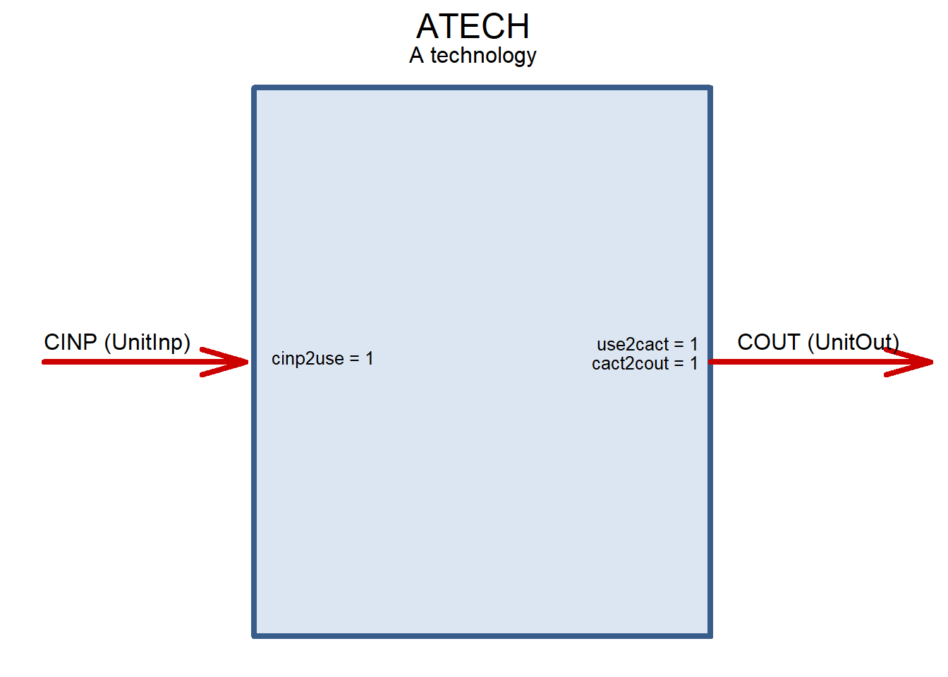
Arrows on the sketch describe commodities flow.
Every technology is characterized by its maximum instant (or nameplate) capacity to produce a commodity(-ies), and its activity in time. capacity is a technological resource, while activity is a usage of the resource. Both can be partially or entirely exogenous or endogenous, meaning their level is defined on the stage of the model formulation by a modeler, or can be a result of the optimization - the model solution.
It is important to identify the main activity commodity of the technology and set units of activity and capacityfor every technology. The relation between capacity and activity units is set by parameter cap2act in the slot @cap2act. The default value of the parameter is equal to 1, meaning that capacity of the technology is measured in annual units, for example in million tones of steel a year.
ATECH@cap2act[1] 1Alternatively, if the technology is a coal power plant with the main electricity (ELC) as the main commodity output, the capacity is normally measured in watts, megawatts or gigawatts. The activity commodity can be simply measured in the main commodity units. Therefore, if electricity in the model is measured in gigawatt hours (“GWh”) and capacity in gigawatts (“GW”) then cap2act is simply a number of hours in the year: cap2act = 8760.
ECOA <- newTechnology(
  name = "ECOA",
  desc = "Coal-fired power plant",
  input = list(
    comm = "COA",
    unit = "PJ"
  ),
  output = list(
    comm = "ELC",
    unit = "GWh"
  ),
  cap2act = 24 * 365
)
ECOA@cap2act
[1] 8760However, if all energy commodities in the model, including ELC are measured in petajoules (“PJ”) then capacity variable and commodity output variable have different units and should be adjusted. There are several ways to do that in the model. First, and the simplest one is to adjust cap2act to the conversion coefficient between the two units. In our case, annual output of 1 GW of installed capacity can produce up to 8760 GWh, that is an equivalent of 31.536 PJ.
ECOA <- update(ECOA,
               cap2act = 24 * 365 * convert(1, from = "GWh", to = "PJ"),
               output = list(comm = "ELC", unit = "PJ") # changing units from GWh
               )
ECOA@cap2act
[1] 31.536Units or electricity in this example should be also changed to “PJ”. Or alternatively the activity of the technology can stay in “PJ” but the output can be converted using cact2cout parameter is slot @ceff as discussed later.
In most cases technological processes are more complicated and have more main inputs, outputs, or associated consumed, produces, or emitted commodities. There are groups of such parameters in energyRt to model different types of relations.
If shares of all inputs or outputs are fixed and the same in every moment of production, they can be modeled as equal main commodities by adding directly to the @input and/or @output slots. Continuing our example of coal power plant, lets add biomass “BIO” co-firing in the inputs.
# Coal only
ECOA@input
comm unit group combustion
1 COA PJ <NA> NA# Adding biomass (BIO)
ECOA <- update(ECOA, input = list(comm = c("COA", "BIO"),
unit = c("PJ", "PJ")))
ECOA@input comm unit group combustion
1 COA PJ <NA> NA
2 BIO PJ <NA> NAdraw(ECOA)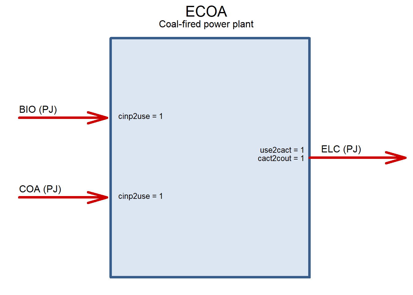
In this example both commodities “COA” and “BIO” are required to produce electricity with this technology. (Efficiency parameters are considered later)
Let’s now assume that the power plant also produces heat (“HEA”) and the ratio between two output commodity is also fixed. To declare HEA as an additional main output it should be declared in the @output slot the same way as for input. co-firing in the inputs.
# Electricity only
ECOA@output
comm unit group
1 ELC PJ <NA># Adding heat (HEA)
ECOA <- update(ECOA, output = list(comm = c("ELC", "HEA"),
unit = c("PJ", "PJ")))
ECOA@output comm unit group
1 ELC PJ <NA>
2 HEA PJ <NA>draw(ECOA)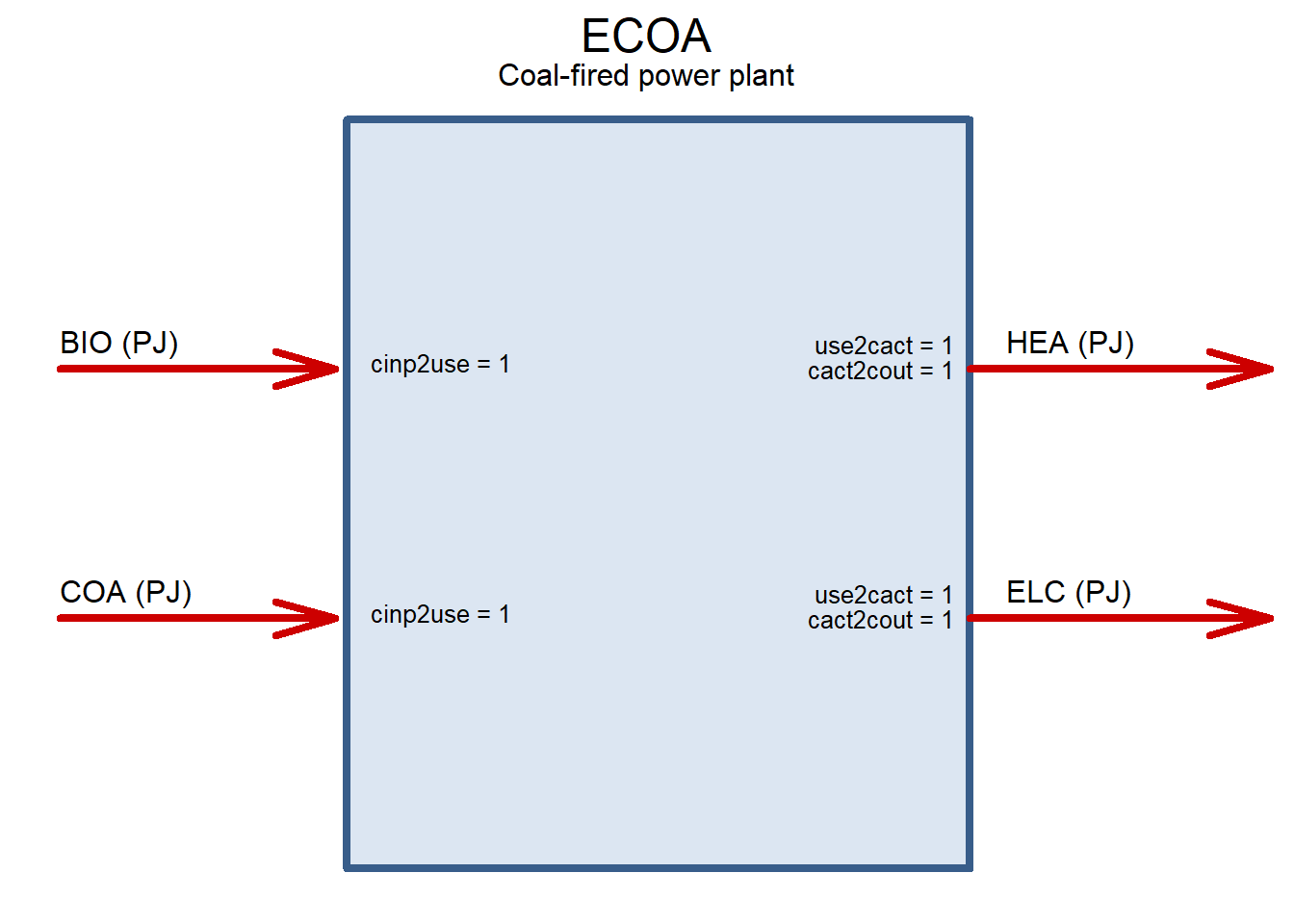
Both output commodities are declared as the main (core) commodities. Sum of their activity will be considered as the activity of the technology. (The required parameters will be set later)
Alternative scenario is when the two commodities can be substitutes. If “BIO” is not available (or too expensive), then “COA” can be used instead and vice versa. To declare substitution between commodities, they should be grouped by adding the same caracter name for the commodities to the group column in the same @input slot.
ECOA <- update(ECOA, input = list(comm = c("COA", "BIO"),
                                  unit = c("PJ", "PJ"),
                                  group = c("i", "i")))
ECOA@input
comm unit group combustion
1 COA PJ i NA
2 BIO PJ i NAdraw(ECOA)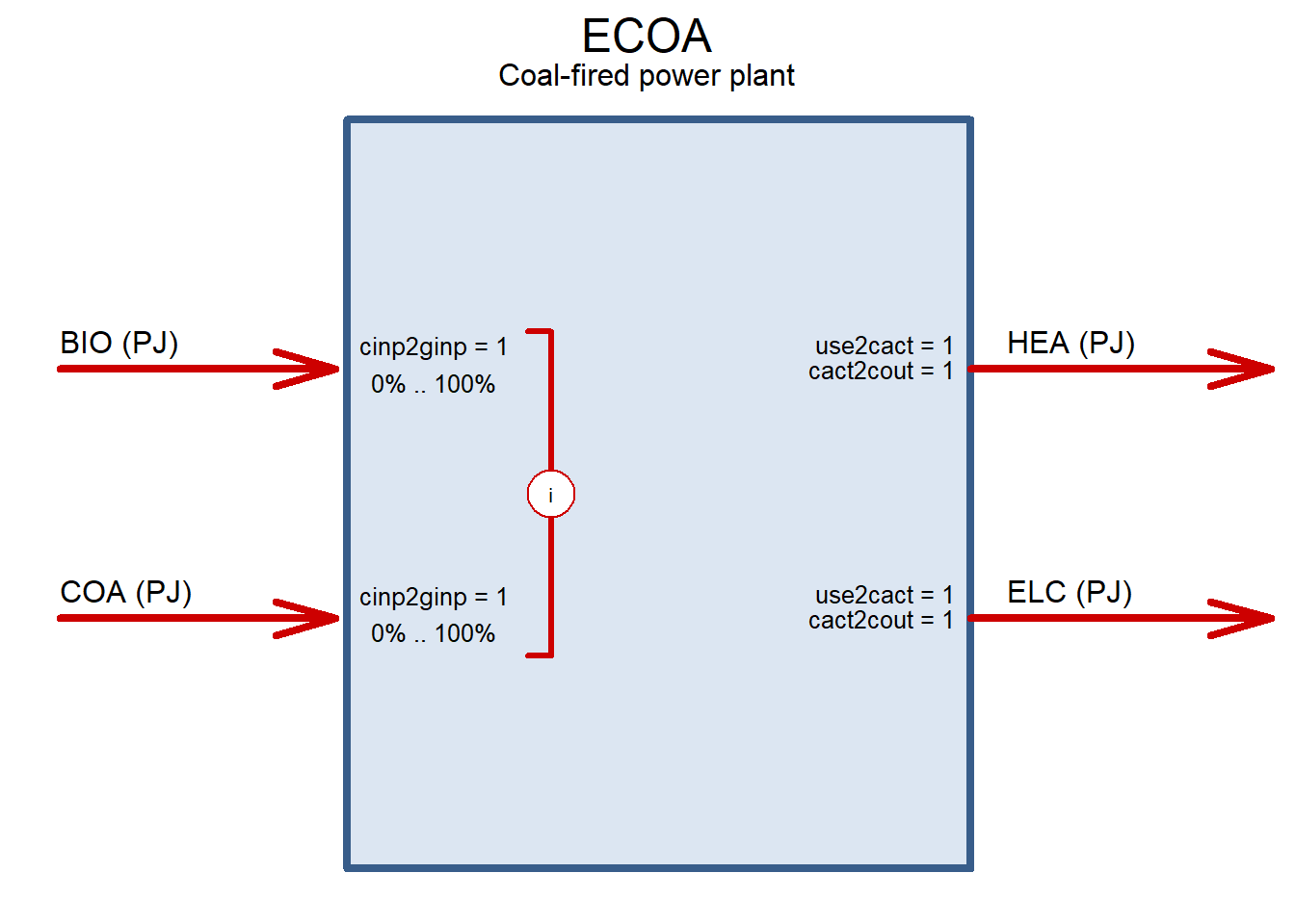
Names of groups can repeat in different technologies, they will not interfere in the model code.
Output commodities can be grouped the same way as input, by assigning a character name of the output group against output commodities in the @output slot. Let’s call the technology differently - combined heat and power plant.
ECOA@output comm unit group
1 ELC PJ <NA>
2 HEA PJ <NA>ECHP <- update(ECOA,
desc = "Coal-fired CHP plant",
output = list(comm = c("ELC", "HEA"),
unit = c("PJ", "PJ"),
group = c("o", "o")))
ECHP@output comm unit group
1 ELC PJ o
2 HEA PJ odraw(ECHP)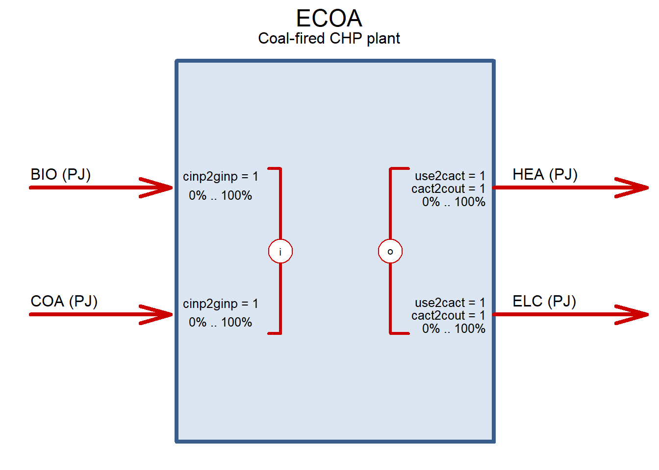
With those settings the technology can equally produce electricity and/or heat in any proportion using coal or biomass or both.
In the example above CHP plan had all efficiency parameters equal to their default value (= 1) meaning that efficiency of the process is equal to 100%. One unit of input (COA or BIO) will produce one unit of output (ELC or HEA). Efficiency parameters for main commodities are stored in @ceff (commodity efficiency) and @geff (group efficiency) slots.
str(ECHP@ceff)'data.frame': 0 obs. of 14 variables:
$ region : chr
$ year : int
$ slice : chr
$ comm : chr
$ cinp2use : num
$ use2cact : num
$ cact2cout: num
$ cinp2ginp: num
$ share.lo : num
$ share.up : num
$ share.fx : num
$ afc.lo : num
$ afc.up : num
$ afc.fx : num str(ECHP@geff)'data.frame': 0 obs. of 5 variables:
$ region : chr
$ year : int
$ slice : chr
$ group : chr
$ ginp2use: num storagerepositorymodelscenariohttps://en.wikipedia.org/wiki/Greenhouse_gas#Global_warming_potential↩︎