[WORK IN PROGRESS]
Map
gis_sf <- cepro_maps$mainland_r34
plot(gis_sf["region"], reset = F, main = "Selected regions")

# keep mainland regions only
gis_sf <- gis_sf %>%
  filter(!grepl("CHN|TW|HK|MO", region))
plot(gis_sf["region"], add = T, col = NA, border = "red", lwd = 1)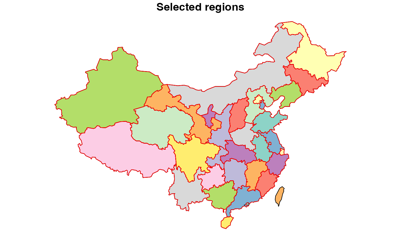
(reg_names <- gis_sf$region)
#>  [1] "XJ" "XZ" "NM" "QH" "SC" "HL" "GS" "YN" "GX" "HN" "SN" "GD" "JL" "HE" "HB"
#> [16] "GZ" "SD" "JX" "HA" "LN" "SX" "AH" "FJ" "ZJ" "JS" "CQ" "NX" "HI" "BJ" "TJ"
#> [31] "SH"
Sub-annual time resolution (calendar)
calendar_full_year <- newCalendar(cepro_timetables$d365_h24)

# subset calendar, selecting 15th day of month
calendar_12d_24h <- newCalendar(
  cepro_timetables$d12_h24,
  year_fraction = sum(cepro_timetables$d12_h24$share))
Commodities
COA <- newCommodity(
  name = "COA",
  desc = "Generic coal",
  emis = list(
    comm = "CO2",
    unit = "kt/GWh",
   emis = convert("kt/PJ", "kt/GWh", 102)
  ),
  slice = "ANNUAL"
)

OIL <- newCommodity(
  name = "OIL",
  desc = "Oil",
  emis = list(
    comm = "CO2",
   unit = "kt/GWh",
    emis = convert("kt/PJ", "kt/GWh", 83)
  ),
  slice = "ANNUAL"
)

GAS <- newCommodity(
  name = "GAS",
  desc = "Generic coal",
  emis = list(
    comm = "CO2",
    unit = "kt/GWh",
    emis = convert("kt/PJ", "kt/GWh", 70)
  ),
  slice = "ANNUAL"
)

BIO <- newCommodity(
  name = "BIO",
  desc = "Generic biomass, all types",
  slice = "ANNUAL"
)

ELC <- newCommodity('ELC', desc = "Electricity", slice = "HOUR")
CO2 <- newCommodity('CO2', desc = "Carbon Dioxide Emissions",  slice = "HOUR")
NUC <- newCommodity("NUC", desc = "Nuclear energy", slice = "ANNUAL")

# Renewable energy, detailed (increases the model size)
# HYD <- newCommodity("HYD", desc = "Hydro energy", slice = "ANNUAL")
# SOL <- newCommodity('SOL', desc = "Solar energy", slice = "ANNUAL")
# WIN <- newCommodity('WIN', desc = "Onshore wind energy", slice = "ANNUAL")
# WIF <- newCommodity('WIF', desc = "Offshore wind energy", slice = "ANNUAL")

# Renewable energy one-for-all (to minimize the model size)
REN <- newCommodity('REN', desc = "All renewables (non-fuels)", slice = "ANNUAL")
Primary Supply
SUP_NUC <- newSupply(
  name = "SUP_NUC",
  commodity = "NUC",
  unit = "GWh",
  availability = list(
    # http://www.world-nuclear.org/information-library/economic-aspects/economics-of-nuclear-power.aspx
    cost = convert("USD/kWh", "MRMB/GWh", .39/100)
  ),
  slice = "ANNUAL"
)

RES_REN <- newSupply(
  name = "RES_REN",
  desc = "Renewable energy (all types)",
  commodity = "REN",
  unit = "GWh",
  slice = "HOUR"
)

SUP_COA <- newSupply(
  name = "SUP_COA",
  desc = "Supply of coal",
  commodity = "COA",
  unit = "PJ",
  # reserve = list(res.up = 1e6),
  availability = list(
    year = c(2010, 2020, 2050),
    # ava.up = c(1000, 2000, 10000),
    cost = c(convert("USD/tce", "MRMB/GWh", c(70, 80, 100) / .7))
  ),
  slice = "ANNUAL"
)

# Bio energy
bio_PJ <- cepro_data$bio_resource_PJ
# Check
all(bio_PJ$region %in% reg_names)
#> [1] TRUE
all(reg_names %in% bio_PJ$region)
#> [1] TRUE

SUP_BIO <- newSupply(
  name = "SUP_BIO",
  desc = "Biomass resource, annual",
  commodity = "BIO",
  unit = "PJ",
  # weather = list(weather = "WEATHER", wava.up = 1),
  availability = data.frame(
    # year = c(2010, 2020, 2050),
    region = bio_PJ$region,
    ava.up = 0.5 * bio_PJ$bio_PJ, # Assumption, 50% for ELC generation
    cost = convert("USD/tce", "MRMB/GWh", 100) # assumption - transaction costs
  ),
  slice = "ANNUAL"
)
Demand
DEM_ELC_FLAT <- newDemand(
  name = "DEM_ELC_FLAT",
  commodity = "ELC",
  unit = "GWh",
  dem = list(
    year = cepro_data$elc_cons_hourly_average_GWh$year,
    region = cepro_data$elc_cons_hourly_average_GWh$region,
    slice = cepro_data$elc_cons_hourly_average_GWh$slice,
    dem = cepro_data$elc_cons_hourly_average_GWh$elc_con_dh_GWh
    )
)
Capacity factors
Solar
a <- ggplot(cepro_maps$sol_GW_max_sf) +
  geom_sf(fill = "lightgrey", data = gis_sf) +
  geom_sf(aes(fill = scf_tl), color = alpha("black", .5)) +
  scale_fill_viridis_c(option = "H", direction = 1) +
  # labs(title = "clastered solar locations") +
  theme_void()
try(a)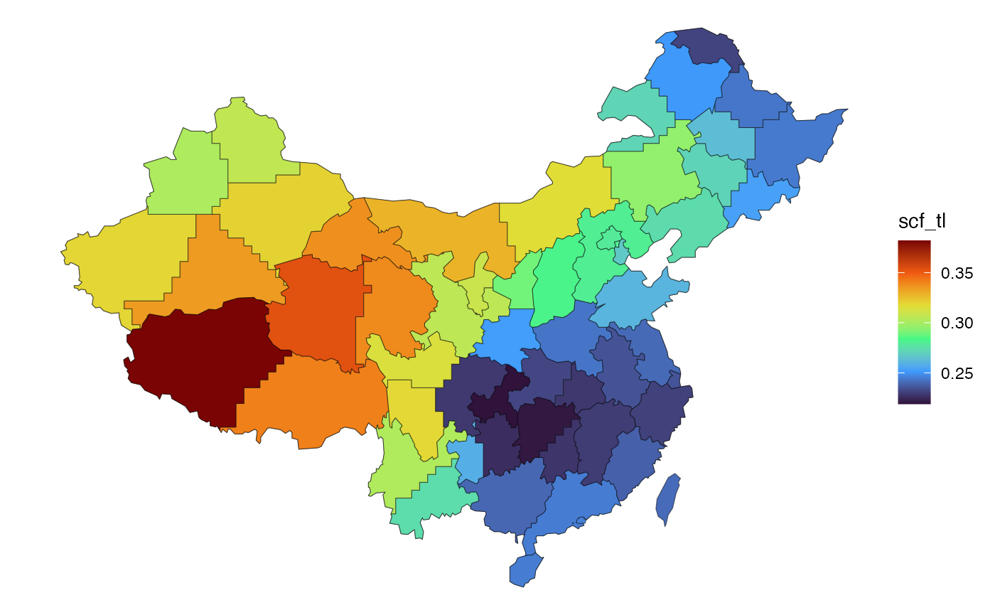
solar <- cepro_maps$sol_GW_max_sf %>%
  mutate(
    weather = paste0("WSOL", formatC(cluster, width = 2, flag = "0")),
    tech_name = paste0("ESOL", formatC(cluster, width = 2, flag = "0")),
    .after = "region"
  )

# cepro_merra_sol_cl

repo_solar_cf <- newRepository("repo_solar_cf")
if (nrow(solar) > 0) {
  for (w in unique(solar$weather)) {
    # stop()
    xi <- filter(solar, weather %in% w)
    x <- cepro_merra_sol_cl %>%
      filter(cluster %in% unique(xi$cluster))
    WSOL <- newWeather(
      name = w,
      desc = "Solar generation profile",
      slice = "HOUR",
      weather = data.frame(
        region = x$region,
        slice = x$slice,
        wval = x$scf_tl
      )
    )
    repo_solar_cf <- add(repo_solar_cf, WSOL); rm(WSOL)
  }
}
repo_solar_cf %>% names()
#> [1] "WSOL01" "WSOL02" "WSOL03" "WSOL04" "WSOL05"
Wind
a <- ggplot(cepro_maps$win_GW_max_sf) +
  geom_sf(fill = "lightgrey", data = gis_sf) +
  geom_sf(aes(fill = wcf100m), color = alpha("black", .5)) +
  scale_fill_viridis_c(option = "H", direction = 1) +
  # labs(title = "clastered solar locations") +
  theme_void()
try(a)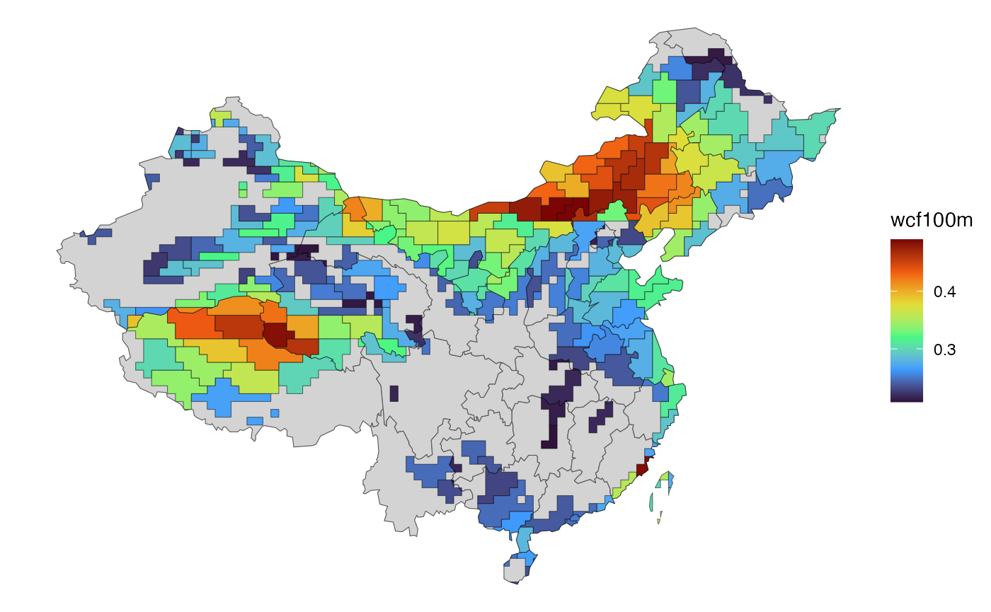
# cepro_merra_win_cl

wind <- cepro_maps$win_GW_max_sf %>%
  mutate(
    weather = paste0("WWIN", formatC(cluster, width = 2, flag = "0")),
    tech_name = paste0("EWIN", formatC(cluster, width = 2, flag = "0")),
    .after = "region"
  ) %>%
  filter(cluster <= 10)
wind$cluster %>% unique()
#>  [1]  1  2  3  4  5  6  7  8  9 10

repo_wind_cf <- newRepository("repo_wind_cf")
if (nrow(wind) > 0) {
  for (w in unique(wind$weather)) {
    # stop()
    xi <- filter(wind, weather %in% w)
    x <- cepro_merra_win_cl %>%
      filter(cluster %in% unique(xi$cluster))
    WWIN <- newWeather(
      name = w,
      desc = "Wind generation profile",
      slice = "HOUR",
      weather = data.frame(
        region = x$region,
        slice = x$slice,
        wval = x$wcf100m
      )
    )
    repo_wind_cf <- add(repo_wind_cf, WWIN); rm(WWIN)
  }
}
repo_wind_cf %>% names()
#>  [1] "WWIN01" "WWIN02" "WWIN03" "WWIN04" "WWIN05" "WWIN06" "WWIN07" "WWIN08"
#> [9] "WWIN09" "WWIN10"Solar
repo_solar_tech <- newRepository("repo_solar_tech")
if (nrow(solar) > 0) {
  for (tch in unique(solar$tech_name)) {
    # cat(tch, "")
    # stop()
    x <- filter(solar, tech_name %in% tch)
    # x <- cepro_merra_sol_cl %>%
    #   filter(cluster %in% unique(xi$cluster))

    tech <- newTechnology(
      name = tch,
      desc = x$tech_name[1],
      # description = paste(x$generators_i, collapse = ", "),
      input = list(comm = "REN", combustion = F),
      output = list(comm = "ELC"),
      cap2act = 24*365,
      olife = list(olife = 25), # for 1-year model & annualized costs,
      weather = list(
        weather = x$weather[1],
        waf.up = 1
      ),
      region = unique(x$region),
      # ceff = list(
      #   region = x$region,
      #   comm = "REN",
      #   cinp2use = 1
      # ),
      fixom = data.frame(
        region = x$region,
        fixom = 3.5/20 # assumption
      ),
      # varom = list(
      #   region = x$region,
      #   varom = x$generators_marginal_cost
      # ),
      # stock = list(
      #   region = x$region,
      #   stock = x$generators_p_nom
      # )
      invcost = list(
        invcost = convert(3.5, "RMB/W", "MRMB/GW")
      ) # overnight
    )
    repo_solar_tech <- add(repo_solar_tech, tech); rm(tech)
  }
}
repo_solar_tech %>% names()
#> [1] "ESOL01" "ESOL02" "ESOL03" "ESOL04" "ESOL05"
draw(repo_solar_tech$ESOL01)
Wind
repo_wind_tech <- newRepository("repo_wind_tech")
if (nrow(wind) > 0) {
  for (tch in unique(wind$tech_name)) {
    # cat(tch, "")
    # stop()
    x <- filter(wind, tech_name %in% tch)
    # x <- cepro_merra_win_cl %>%
    #   filter(cluster %in% unique(xi$cluster))

    tech <- newTechnology(
      name = tch,
      desc = x$tech_name[1],
      # description = paste(x$generators_i, collapse = ", "),
      input = list(comm = "REN", combustion = F),
      output = list(comm = "ELC"),
      cap2act = 24*365,
      olife = list(olife = 25), # for 1-year model & annualized costs
      weather = list(
        weather = x$weather[1],
        waf.up = 1
      ),
      region = unique(x$region),
      # ceff = list(
      #   region = x$region,
      #   comm = "REN",
      #   cinp2use = 1
      # ),
      fixom = data.frame(
        region = x$region,
        fixom = 6.7/20 # assumption
      ),
      # varom = list(
      #   region = x$region,
      #   varom = x$generators_marginal_cost
      # ),
      # stock = list(
      #   region = x$region,
      #   stock = x$generators_p_nom
      # )
      invcost = list(
        invcost = convert(6.7, "RMB/W", "MRMB/GW")
      ) # overnight
    )
    repo_wind_tech <- add(repo_wind_tech, tech); rm(tech)
  }
}
repo_wind_tech %>% names()
#>  [1] "EWIN01" "EWIN02" "EWIN03" "EWIN04" "EWIN05" "EWIN06" "EWIN07" "EWIN08"
#>  [9] "EWIN09" "EWIN10"
draw(repo_wind_tech@data[[1]])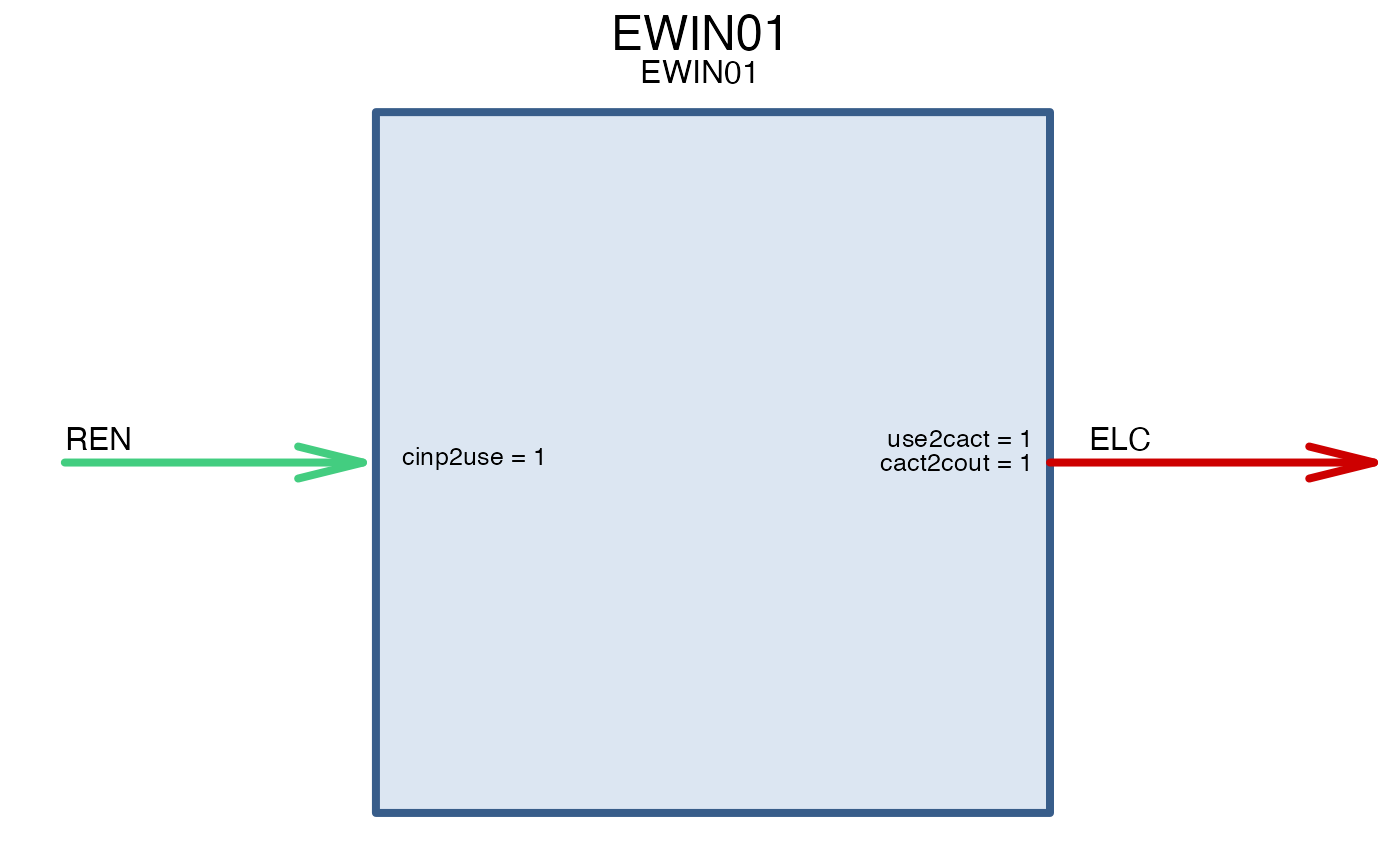
Storage
STGELC <- newStorage(
  name = 'STGELC',
  commodity = 'ELC',
  desc = "1-hours storage (battery)",
  cap2stg = 1, # In PJ convert("GWh", "PJ"),
  # afa = list(year = 2020, slice = "m06h23", afa.lo = .5),
  olife = list(olife = 15),
  # invcost = list(invcost = convert("USD/MWh", "MRMB/PJ", 180)), # Assumption
  # invcost = list(invcost = convert("USD/kWh", "MRMB/PJ", 100)), # See IRENA 2030 (from 77 to 574, p.77)
  invcost = list(invcost = convert("USD/kWh", "MRMB/GWh", 300)), # See IRENA 2030 (from 77 to 574, p.77)
  seff = data.frame(inpeff = 0.8) # stgeff = .9,
)Model 100% Ren
repo_ren <- newRepository("repo_ren") %>%
  add(
    REN, ELC,
    RES_REN,
    repo_solar_cf,
    repo_solar_tech,
    # repo_wind_cf,
    # repo_wind_tech,
    LOSTLOAD,
    STGELC,
    DEM_ELC_FLAT
  )

length(repo_ren)
#> [1] 16
print(repo_ren)
#> repository 'repo_ren': 16 objects.
#>             name      class
#>  1:          REN  commodity
#>  2:          ELC  commodity
#>  3:      RES_REN     supply
#>  4:       WSOL01    weather
#>  5:       WSOL02    weather
#>  6:       WSOL03    weather
#>  7:       WSOL04    weather
#>  8:       WSOL05    weather
#>  9:       ESOL01 technology
#> 10:       ESOL02 technology
#> 11:       ESOL03 technology
#> 12:       ESOL04 technology
#> 13:       ESOL05 technology
#> 14:     LOSTLOAD     import
#> 15:       STGELC    storage
#> 16: DEM_ELC_FLAT     demand
names(repo_ren)
#>  [1] "REN"          "ELC"          "RES_REN"      "WSOL01"       "WSOL02"
#>  [6] "WSOL03"       "WSOL04"       "WSOL05"       "ESOL01"       "ESOL02"
#> [11] "ESOL03"       "ESOL04"       "ESOL05"       "LOSTLOAD"     "STGELC"
#> [16] "DEM_ELC_FLAT"
summary(repo_ren)
#>  commodity     demand     import    storage     supply technology    weather
#>          2          1          1          1          1          5          5

# Adjust annual parameters for partial year solution
# (temporary solution - until implementation of the method in energyRt)
# repo <- fract_year_adj_repo(repo, SUBSET_HOURS)

# repo_subset <- subset_slices_repo(repo, SLICE_SUBSET, YDAY_SUBSET)

# model-class object
mod <- newModel(
  name = 'CEPRO_ren',
  desc = "CEPRO renewables only",
  ## in case of infeasibility, `dummy` variables can be added
  # debug = data.frame(#comm = "ELC",
  #                    dummyImport = 1e6,
  #                    dummyExport = 1e6),
  region = unique(gis_sf$region),
  discount = 0.05,
  calendar = calendar_full_year,
  data = repo_ren)

# Check the model time-slices
mod@config@calendar@timetable %>% as.data.table()
#>       ANNUAL YDAY HOUR    slice        share
#>    1: ANNUAL d001  h00 d001_h00 0.0001141553
#>    2: ANNUAL d001  h01 d001_h01 0.0001141553
#>    3: ANNUAL d001  h02 d001_h02 0.0001141553
#>    4: ANNUAL d001  h03 d001_h03 0.0001141553
#>    5: ANNUAL d001  h04 d001_h04 0.0001141553
#>   ---
#> 8756: ANNUAL d365  h19 d365_h19 0.0001141553
#> 8757: ANNUAL d365  h20 d365_h20 0.0001141553
#> 8758: ANNUAL d365  h21 d365_h21 0.0001141553
#> 8759: ANNUAL d365  h22 d365_h22 0.0001141553
#> 8760: ANNUAL d365  h23 d365_h23 0.0001141553

mod <- setHorizon(mod, 2015, 1)
mod@config@horizon # check
#> An object of class "horizon"
#> Slot "desc":
#> character(0)
#>
#> Slot "period":
#> [1] 2015
#>
#> Slot "intervals":
#>    start  mid  end
#> 1:  2015 2015 2015
Scenarios
Base ren
scen_ren_sub <- interpolate(mod, calendar_12d_24h)
# scen_ren <- interpolate(mod)
# scen_gms <- write_sc(
#   scen_ren_sub,
#   # solver = "gams", # see "solver_options_generic.r" file
#   solver = GAMS_barrier,
#   # solver = GAMS_new_maps,
#   tmp.dir = file.path("tmp", "ren_test"))
#
# scen_gms <- solve(scen_gms, wait = F)
# scen_gms <- read(scen_gms)

scen_jump <- write_sc(
  scen_ren_sub,
  # solver = "JuMP", # see "solver_options_generic.r" file
  # solver = GAMS_barrier_cbc,
  # solver = GAMS_new_maps,
  tmp.dir = file.path("tmp", "ren_test_julia"))
scen_jump <- solve(scen_jump, wait = F)
[tbc..]