Installation
merra2ools is an R library and a dataset. It is
assumed that R version >=4.0 is pre-installed. (Rtools
is also required on Windows to build this and several other packages
from source or GitHub). It is also recommended (though it is not
required) to use RStudio or
other IDE for R. merra2ools depends on several R-packages
which (if not yet available on your system) will be installed along with
the merra2ools installation (see the package DESCRIPTION
for details). The package also requires its dataset to be downloaded
separately from the installation of the package (see below). Though
merra2ools package can operate without the dataset (for
estimation capacity factors, solar geometry, etc.), the supplied data
should be formatted in the same way as it is expected by the package
functions.
merra2sample is 12-days example of the the
merra2ools subset (41 years), 21st-day of each month of
2010. It can installed directly from GitHub, and used for quick checks
of the data and its format; it is also used to build vignettes
(articles) of merra2ools package. Since the example dataset
has considerable size for R-packages (~0.5Gb) and mostly repeats the
main dataset, it is saved as a separate package.
pkg <- function() rownames(installed.packages()) # returns names of installed packages
# Installation of `merra2ools` package
if (!("remotes" %in% pkg())) install.packages("remotes")
if (!("merra2ools" %in% pkg())) remotes::install_github("energyRt/merra2ools", dependencies = TRUE)
if (!("merra2sample" %in% pkg())) remotes::install_github("energyRt/merra2sample")
# Packages used in the vignette
if (!("rnaturalearthhires" %in% pkg()))
  devtools::install_github("ropensci/rnaturalearthhires")
if (!("scales" %in% pkg())) install.packages("scales")
if (!("cowplot" %in% pkg())) install.packages("cowplot")
if (!("kableExtra" %in% pkg())) install.packages("kableExtra")
merra2ools dataset (~270Gb) can be
downloaded from https://doi.org/10.5061/dryad.v41ns1rtt,
unziped in a dedicated directory on an internal or external hard-drive,
and configured as described below.
Setting up
Loading packages used in the vignette.
Checking if the dataset is connected.
check_merra2()
#> 492 merra2ools data-files found
Connecting the dataset (if not yet connected)
check_merra2("PATH TO THE DOWNLOADED DATA") # check if the data in the directory
set_merra2_options(merra2.dir = "PATH TO THE DOWNLOADED DATA") # safe the path
get_merra2_dir()  # check if the path is saved
check_merra2(detailed = T)
Accessing the data
The database is organized in monthly files in fst
format. There are two functions to read a whole file
(read_merra_file()) or read a subset for specified
locations and time period (get_merra2_subset()). Both
functions provide an option to read the dataset in the scaled format, in
reported units (default) or “raw” format (as integers - the way it is
stored).
x <- read_merra_file("202012", as_integers = TRUE)| UTC | locid | W10M.e1 | W50M.e1 | WDIR.e_1 | T10M.C | SWGDN | ALBEDO.e2 | PRECTOTCORR.kg_m2_h.e1 | RHOA.e2 |
|---|---|---|---|---|---|---|---|---|---|
| 2020-12-01 00:30:00 | 1 | 33 | 47 | 5 | -35 | 421 | 80 | 0 | 99 |
| 2020-12-01 00:30:00 | 2 | 33 | 47 | 5 | -35 | 421 | 80 | 0 | 99 |
| 2020-12-01 00:30:00 | 3 | 33 | 47 | 5 | -35 | 421 | 80 | 0 | 99 |
| 2020-12-01 00:30:00 | 4 | 33 | 47 | 5 | -35 | 421 | 80 | 0 | 99 |
| 2020-12-01 00:30:00 | 5 | 33 | 47 | 5 | -35 | 421 | 80 | 0 | 99 |
x <- get_merra2_subset(from = "20201130 01", to = "20201201 23")| UTC | locid | W10M.e1 | W50M.e1 | WDIR.e_1 | T10M.C | SWGDN | ALBEDO.e2 | PRECTOTCORR.kg_m2_h.e1 | RHOA.e2 |
|---|---|---|---|---|---|---|---|---|---|
| 2020-12-01 00:30:00 | 1 | 33 | 47 | 5 | -35 | 421 | 80 | 0 | 99 |
| 2020-12-01 00:30:00 | 2 | 33 | 47 | 5 | -35 | 421 | 80 | 0 | 99 |
| 2020-12-01 00:30:00 | 3 | 33 | 47 | 5 | -35 | 421 | 80 | 0 | 99 |
| 2020-12-01 00:30:00 | 4 | 33 | 47 | 5 | -35 | 421 | 80 | 0 | 99 |
| 2020-12-01 00:30:00 | 5 | 33 | 47 | 5 | -35 | 421 | 80 | 0 | 99 |
Locations identifiers
Every data-point in the used MERRA-2 collections (see the dataset
description) is associated with coordinates and time. The original
MERRA-2 files have index-variables V1, V2, and
V3 to identify longitude, latitude, and time (hour)
dimensions respectively. For convenience, a location identifier
locid has been generated as a Kronecker product of
V1 and V2. The locid identifier
is used as the key variable of MERRA-2 locations, instead of
V1 and V2. The time identifier
(V3 - hour) is combined with the year, month, and day in
UTC key variable. The total number of location points in
MERRA-2 is 207,936 (576 X 361). The identifier is saved in the
merra2ools package \data directory and can be
called with data function (data("locid")) or
directly locid.
# Ways to call `locid` data.frame
data("locid")
merra2ools::locid
locid| lon | lat | locid | V1 | V2 | FRLAKE | FRLAND | FRLANDICE | FROCEAN | PHIS | SGH |
|---|---|---|---|---|---|---|---|---|---|---|
| -180.000 | -90 | 1 | 1 | 1 | 0 | 0 | 1 | 0.0000000 | 27576.33 | 11.49101 |
| -179.375 | -90 | 2 | 2 | 1 | 0 | 0 | 1 | 0.0000000 | 27576.33 | 11.49101 |
| -178.750 | -90 | 3 | 3 | 1 | 0 | 0 | 1 | 0.0000000 | 27576.33 | 11.49101 |
| 178.125 | 90 | 207934 | 574 | 361 | 0 | 0 | 0 | 0.9999962 | 0.00 | 0.00000 |
| 178.750 | 90 | 207935 | 575 | 361 | 0 | 0 | 0 | 0.9999962 | 0.00 | 0.00000 |
| 179.375 | 90 | 207936 | 576 | 361 | 0 | 0 | 0 | 0.9999962 | 0.00 | 0.00000 |
code
lon <- unique(locid$lon)
head(lon, 10)
length(lon)

lat <- unique(locid$lat)
head(lat, 10)
length(lat)

lo <- unique(c(seq(-180, max(lon), by = 30), max(lon))) %>% sort()
la <- seq(-90, 90, by = 15)

locid_sample <- filter(locid, lon %in% lo, lat %in% la)
world_map <- rnaturalearth::ne_countries(scale = "small", returnclass = "sf")

fig.locid <- ggplot() +
  geom_sf(fill = "wheat", alpha = .75, colour = NA, size = 0.25, data = world_map) +
  theme_bw() +
  geom_rect(aes(xmin = xmin, xmax = xmax, ymin = ymin, ymax = ymax),
    data = data.frame(xmin = -180, xmax = 180, ymin = -90, ymax = 90),
    alpha = .5, fill = NA, colour = "grey85") +
  geom_point(aes(x = lon, y = lat), data = locid_sample, size = 1, colour = "red") +
  geom_text(aes(x = lon, y = lat, label = locid), data = locid_sample,
             position = position_nudge(y = 4),
             alpha = 0.75,
             size = unit(3, "lines")) +
  scale_x_continuous(breaks = ceiling(lo), minor_breaks = ceiling(lo)) +
  scale_y_continuous(breaks = round(la), minor_breaks = ceiling(la)) +
  labs(x = "lon") +
  coord_sf(xlim = c(-190, 190), ylim = c(-95, 95)) +
  # labs(x = "lon", title = "Location ID (`locid`) layout of MERRA-2 subset") +
  theme(plot.title = element_text(hjust = 0.5),
        axis.text = element_text(family = 'arial'))

ggsave("images/locid_map2.png", fig.locid, width = 9, height = 5.)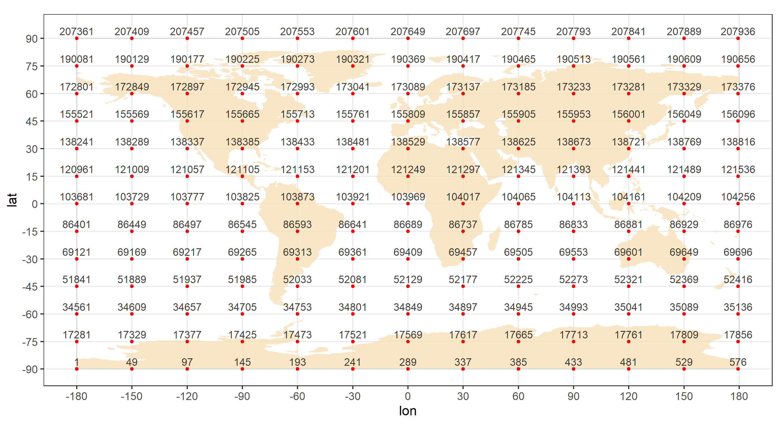
locid_map
Matching locid with a map
Location identifiers in merra2ools dataset can be seen
as spatial points or centers (centroids) of a spatial grid or spatial
polygons. Subsetting locid for a particular geographical
region can be done using a “map” of the region in
SpatialPolygonsDataFrame format (spdf).
Function get_locid offers two alternative criteria of
selecting locids is implemented in get_locid
function:
* locid as a spatial points overlay the map’s
spatial polygons (method = “points”);
* locid as a spatial polygon intersect with the
map’s spatial polygons (method = “intersect”).
Three examples below compare subsetting with the two methods for three
different regions/countries.
Example 1. Florida, USA
# US-map
usa_sf <- rnaturalearth::ne_states(iso_a2 = "us", returnclass = "sf")

# Subset Florida map
florida_sf <- usa_sf[usa_sf$name_en == "Florida",]

# location IDs, two methods
locid_fl_p <- get_locid(florida_sf, method = "points")
locid_fl_i <- get_locid(florida_sf, method = "polygons")

# MERRA-2 grid for the selected `locid's`
locid_fl_grid <- get_merra2_grid("poly", locid = locid_fl_i)

# Plot
a <- ggplot() +
  geom_sf(data = florida_sf, fill = "wheat") +
  geom_sf(data = locid_fl_grid, color = "darkgrey", fill = NA) +
  geom_point(aes(lon, lat), data = locid[locid_fl_p,], color = "red", shape = 16) +
  geom_point(aes(lon, lat), data = locid[locid_fl_i,], color = "red", shape = 1) +
  theme_bw() + labs(x = "", y = "")
ggsave("images/example1_florida_locids.png", a, width = 5, height = 5)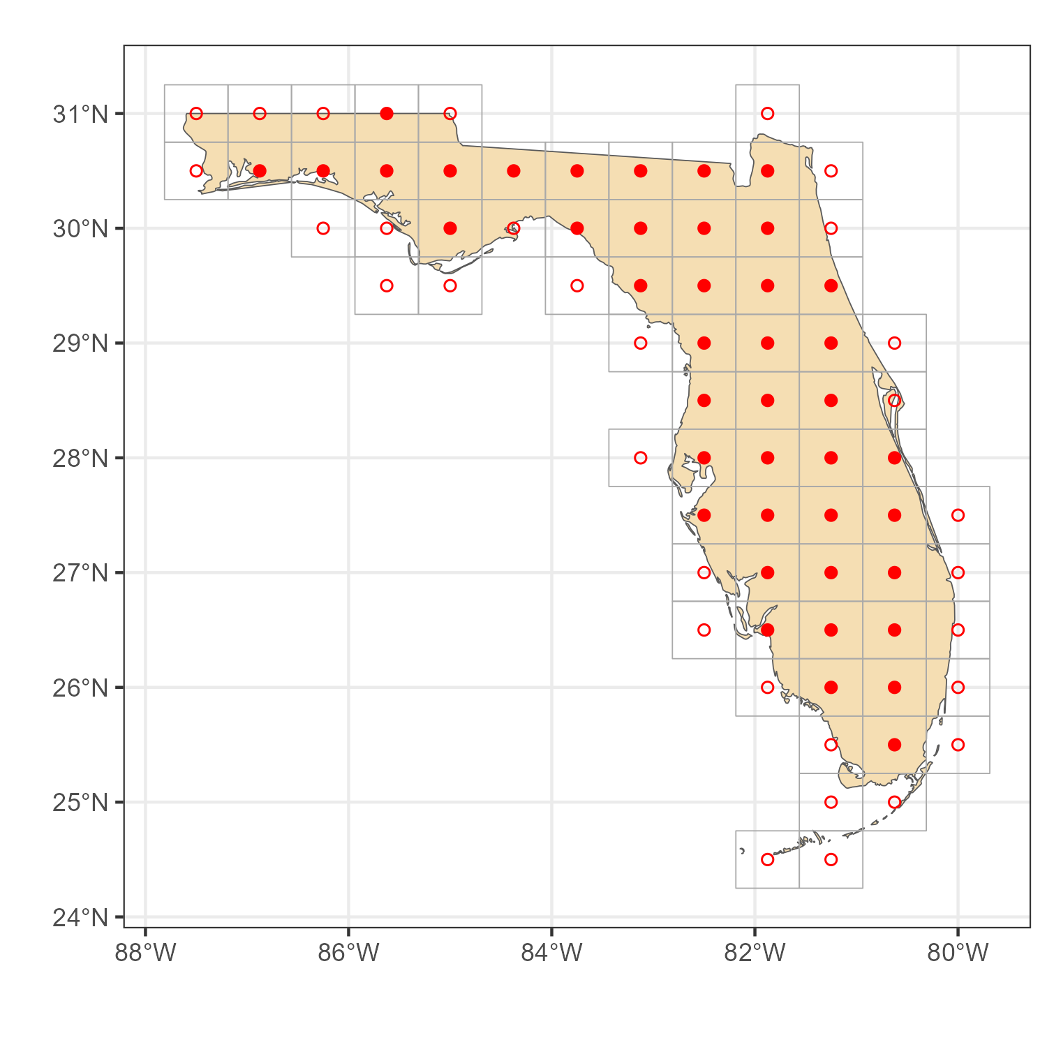
MERRA-2 locations for Florida
Example 2. Iceland
code
# Map
iceland_sf <- rnaturalearth::ne_countries(country = "iceland", scale = "large",
                                          returnclass = "sf")

# location IDs, two methods
locid_isl_p <- get_locid(iceland_sf, method = "points")
locid_isl_i <- get_locid(iceland_sf, method = "poly")

# MERRA-2 grid for the selected `locid's`
locid_isl_grid <- get_merra2_grid("poly", locid = locid_isl_i)

# Plots
a <- ggplot() +
  geom_sf(data = iceland_sf, fill = "wheat") +
  geom_sf(data = locid_isl_grid, color = "darkgrey", fill = NA) +
  geom_point(aes(lon, lat), data = locid[locid_isl_p,], color = "red", shape = 16) +
  geom_point(aes(lon, lat), data = locid[locid_isl_i,], color = "red", shape = 1) +
  theme_bw() + labs(x = "", y = "")
ggsave("images/example2_iceland_locids.png", a, width = 5, height = 5)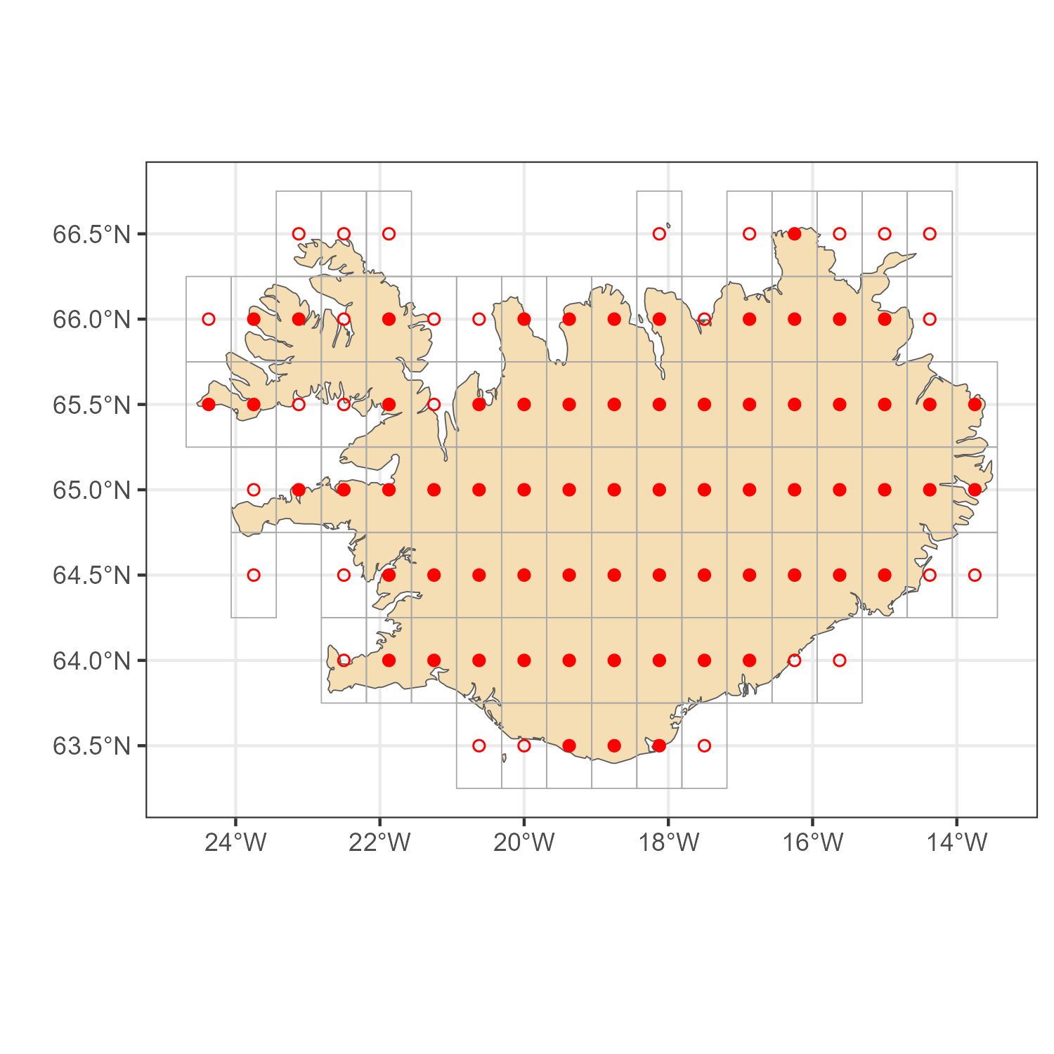
MERRA-2 locations for Iceland
Example 3. Kenya
code
# Map
kenya_sf <- rnaturalearth::ne_countries(country = "kenya", returnclass = "sf")

# location IDs, two methods
locid_ken_p <- get_locid(kenya_sf, method = "points")
locid_ken_i <- get_locid(kenya_sf, method = "poly")

# MERRA-2 grid for the selected `locid's`
locid_ken_grid <- get_merra2_grid("poly", locid = locid_ken_i)

# Plot
a <- ggplot() +
  geom_sf(data = kenya_sf, fill = "wheat") +
  geom_sf(data = locid_ken_grid, color = "darkgrey", fill = NA) +
  geom_point(aes(lon, lat), data = locid[locid_ken_p,], color = "red", shape = 16) +
  geom_point(aes(lon, lat), data = locid[locid_ken_i,], color = "red", shape = 1) +
  theme_bw() + labs(x = "", y = "")
ggsave("images/example3_kenya_locids.png", a, width = 5, height = 5)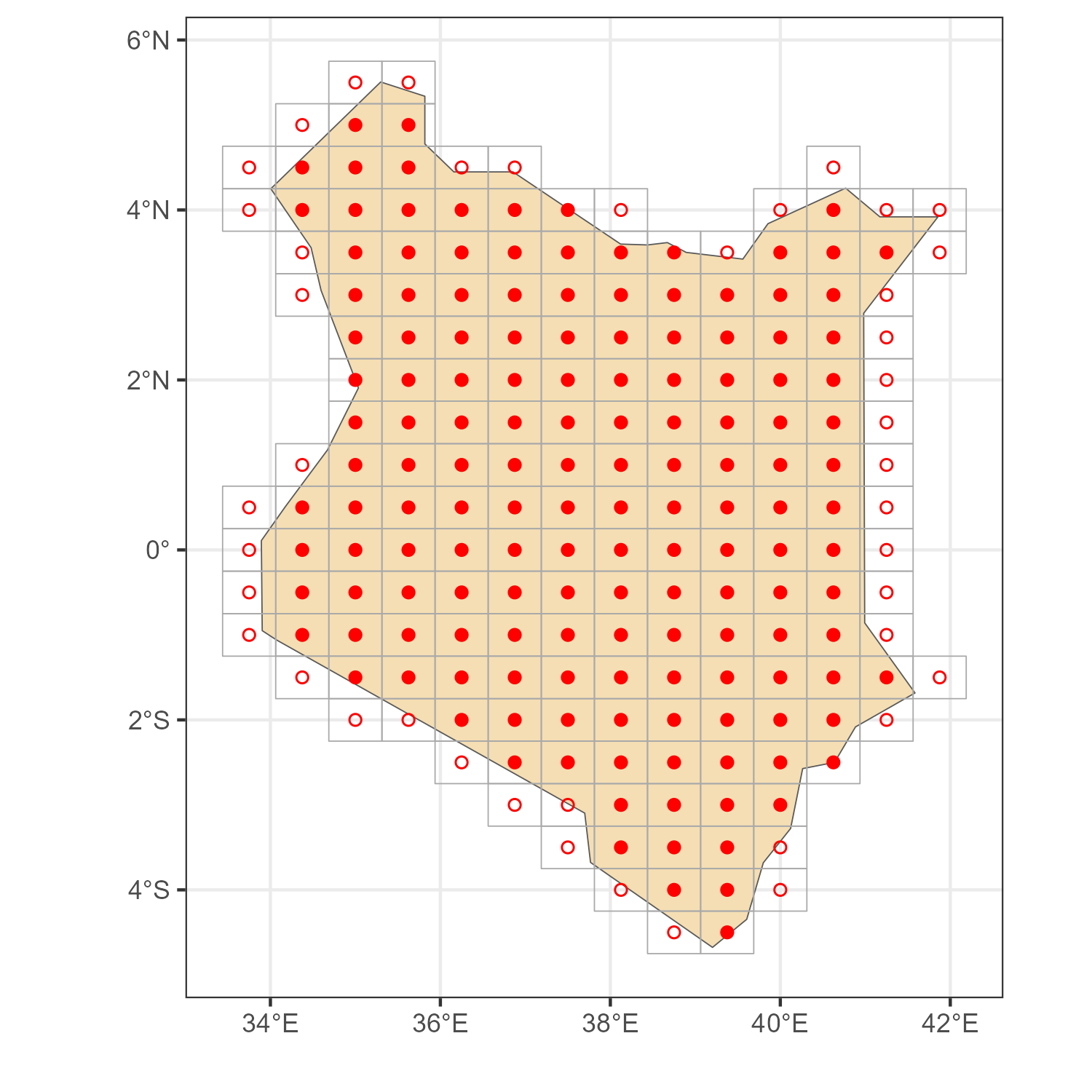
MERRA-2 locations for Kenya
Get MERRA-2 subset
merra_fl <- get_merra2_subset(locid = locid_fl_i,
                              from = "20190101 00", to = "20191231 23",
                              tz = "US/Eastern")

merra_isl <- get_merra2_subset(locid = locid_isl_i,
                               from = "20190101 00", to = "20191231 23",
                               tz = "Atlantic/Reykjavik")

merra_ken <- get_merra2_subset(locid = locid_ken_i,
                               from = "20190101 00", to = "20191231 23",
                               tz = "Africa/Nairobi")
Wind power
Estimation of wind power capacity factors (CF) for the first example - Florida.
# Estimate capacity factors
merra_fl <- fWindCF(merra_fl, height = 150)

# Annual averages
win_fl_y <- merra_fl %>% # annual averages
  group_by(locid) %>%
  summarise(win150af = mean(win150af, na.rm = T)) %>%
  add_merra2_grid()
Cluster locations
We can also cluster locations based on correlation of certain timeseries across locations.
# Cluster locations based on correlation
win_fl_cl <- cluster_locid(
  merra_fl,
  varname = "win150af",
  locid_info = locid_fl_grid,
  max_loss = .05,
  verbose = T)


tol_level <- .10 # 10%
# tol_level <- .05 # 5%

# Select clusters with {tol_level}% tolerance (loss of standard deviation)
win_fl_cl_k <- win_fl_cl %>%
    filter(sd_loss <= tol_level) %>%
    mutate(k_min = (k == min(k))) %>% ungroup() %>%
    filter(k_min) %>% select(-k_min)
code
# Cluster-loss figure
win_fl_cl_kk <- win_fl_cl %>%
  group_by(k) %>%
  summarise(sd_loss = max(sd_loss), N = max(N), .groups = "drop")

locid_win_cl_k_i <- win_fl_cl_k %>%
  group_by(k) %>%
  summarise(sd_loss = max(sd_loss), N = max(N), .groups = "drop")

a <- ggplot(win_fl_cl_kk) +
  geom_line(aes(k, sd_loss), color = "dodgerblue", linewidth = 1.5) +
  geom_point(aes(k, sd_loss), color = "red", data = locid_win_cl_k_i) +
  geom_hline(yintercept = tol_level, color = "red", linetype = 2) +
  scale_y_continuous(labels = scales::percent, limits = c(0, NA)) +
  # scale_x_continuous(breaks = rev_integer_breaks(5)) +
  labs(x = "Number of clusters (k)", y = "loss, % of s.d.") +
  theme_bw()
ggsave("images/example1_florida_wind_clusters.png", a, width = 4.5,
       height = 3)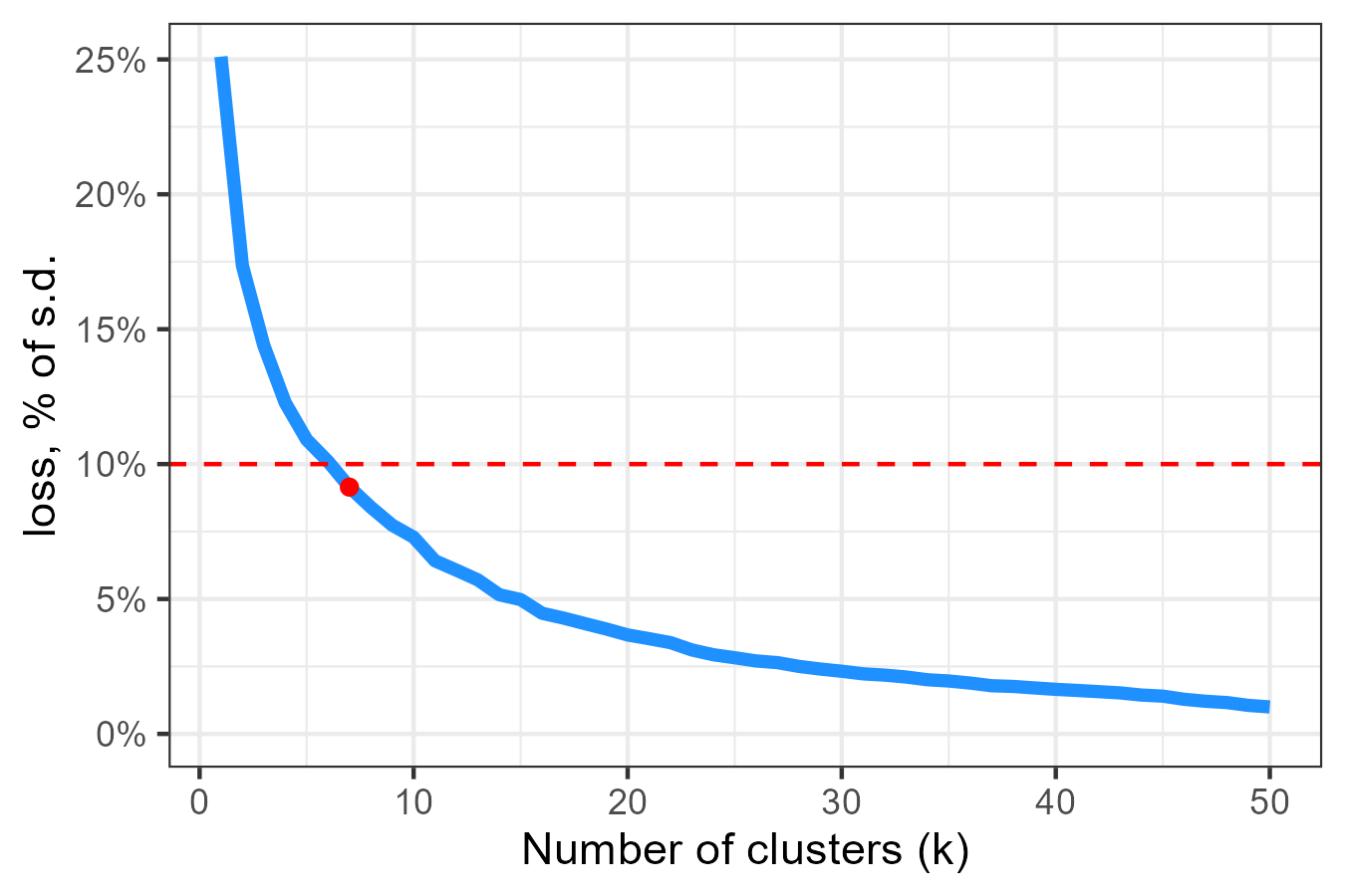
Loss of information as a function of number of clusters
code
win_fl_cl_sf <- locid_fl_grid %>%
  st_make_valid() %>%
  left_join(
    select(win_fl_cl_k, any_of(c("locid", "cluster")))
    ) %>%
  filter(!is.na(cluster)) %>%
  mutate(cluster = factor(cluster))

a <- ggplot(win_fl_cl_sf) +
  geom_sf(fill = "lightgrey", data = florida_sf) +
  geom_sf(aes(fill = cluster), color = NA) +
  geom_sf(color = alpha("black", 1), fill = NA, data = florida_sf) +
  scale_fill_viridis_d(option = "H", direction = 1, name = "Cluster") +
  labs(title = paste0("Clustered wind sites by region",
                      ", sd_loss <= ", tol_level * 100, "%")) +
  theme_bw()
a
ggsave("images/example1_florida_wind_clusters_map.png", a,
       width = 5, height = 5)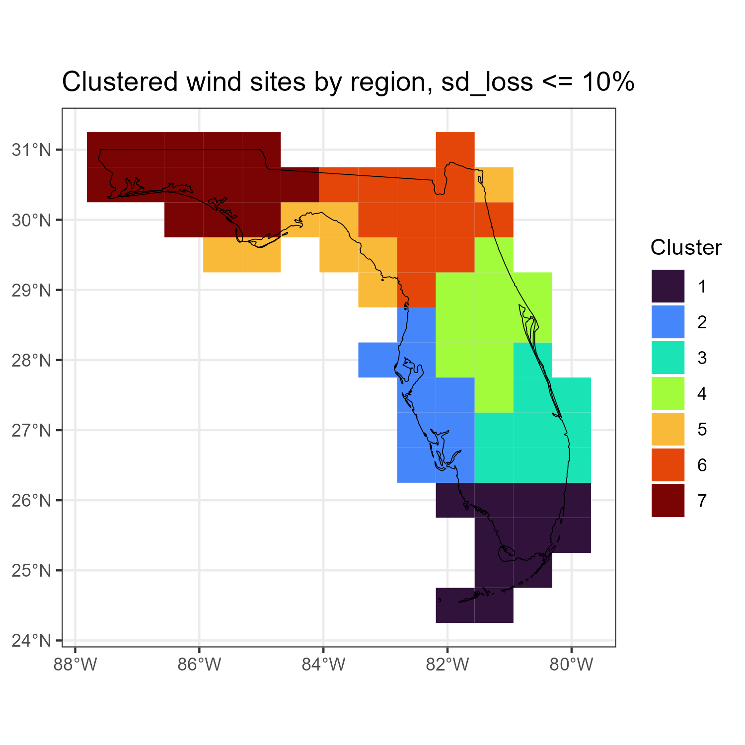
Clustered location based on correlation of wind capacity factors
Solar power
Estimation of Plane of Array Irradiance (POA) for fixed tilted (fl) array-systems for Florida
# Estimate POA
merra_fl <- merra_fl %>% fPOA(array.type = "fl")

# Annual averages
poa_fl_y <- merra_fl %>%
  group_by(locid) %>%
  summarise(POA.fl = sum(POA.fl, na.rm = T)/365/1e3) %>%
add_merra2_grid() code
Iceland
# Estimate POA
merra_isl <- merra_isl %>% fPOA(array.type = "fl")

# Annual averages
poa_isl_y <- merra_isl %>%
  group_by(locid) %>%
  summarise(POA.fl = sum(POA.fl, na.rm = T)/365/1e3) %>%
  add_merra2_grid()
Kenya
# Estimate POA
merra_ken <- merra_ken %>% fPOA(array.type = "fl")

# Annual averages
poa_ken_y <- merra_ken %>%
  group_by(locid) %>%
  summarise(POA.fl = sum(POA.fl, na.rm = T)/365/1e3) %>%
  add_merra2_grid()
Comparative figure
To use the same scale,
wnd_range <- range(win_fl_y$win150af, win_isl_y$win150af, win_ken_y$win150af)
wnd_breaks <- scales::breaks_pretty(5)(wnd_range)
wnd_range <- range(wnd_breaks)

poa_range <- range(poa_fl_y$POA.fl, poa_isl_y$POA.fl, poa_ken_y$POA.fl)
poa_breaks <- scales::breaks_pretty(5)(poa_range)
poa_range <- range(poa_breaks)
# Plot capacity factor variable on map
cf_plot <- function(
  data, gis_sf, var_name, brakes,
  labels = brakes, limits = range(brakes), legend_name = var_name,
  viridis_palette = "viridis", border_colour = alpha("white", .5),
  legend_position = "none") {

  ggplot() +
  geom_sf(aes(fill = .data[[var_name]]), data = data) +
  geom_sf(data = gis_sf, fill = NA, colour = border_colour) +
  scale_fill_viridis_c(
    breaks = brakes, labels = labels, limits = limits, name = legend_name,
    option = viridis_palette) +
  theme_bw() +
    theme(legend.position = legend_position) +
  theme(plot.margin = margin(0.5, 0.0, 0.0, 0.0, "cm")) +
  labs(x = "", y = "")

}

# Combine plots into one
plot_grid(
  cf_plot(win_fl_y, florida_sf, "win150af", wnd_breaks),
  cf_plot(win_isl_y, iceland_sf, "win150af", wnd_breaks),
  cf_plot(win_ken_y, kenya_sf, "win150af", wnd_breaks,
          legend_position = "right", legend_name = "Wind\nCF"),
  # NULL, NULL, NULL,
  cf_plot(poa_fl_y, florida_sf, "POA.fl", poa_breaks, viridis_palette = "plasma"),
  cf_plot(poa_isl_y, iceland_sf, "POA.fl", poa_breaks, viridis_palette = "plasma"),
  cf_plot(poa_ken_y, kenya_sf, "POA.fl", poa_breaks, viridis_palette = "plasma",
          legend_position = "right", legend_name = "POA\nkW/day"),
  # rel_heights = c(1, -.3, 1),
  ncol = 3, rel_widths = c(1, 1.3, 1.17),
  labels = c("Florida", "Iceland", "Kenya"), hjust = c(-1.6, -1.9, -1.6)
)
ggsave2("images/cf_group.png", width = 8, height = 5, dpi = 200)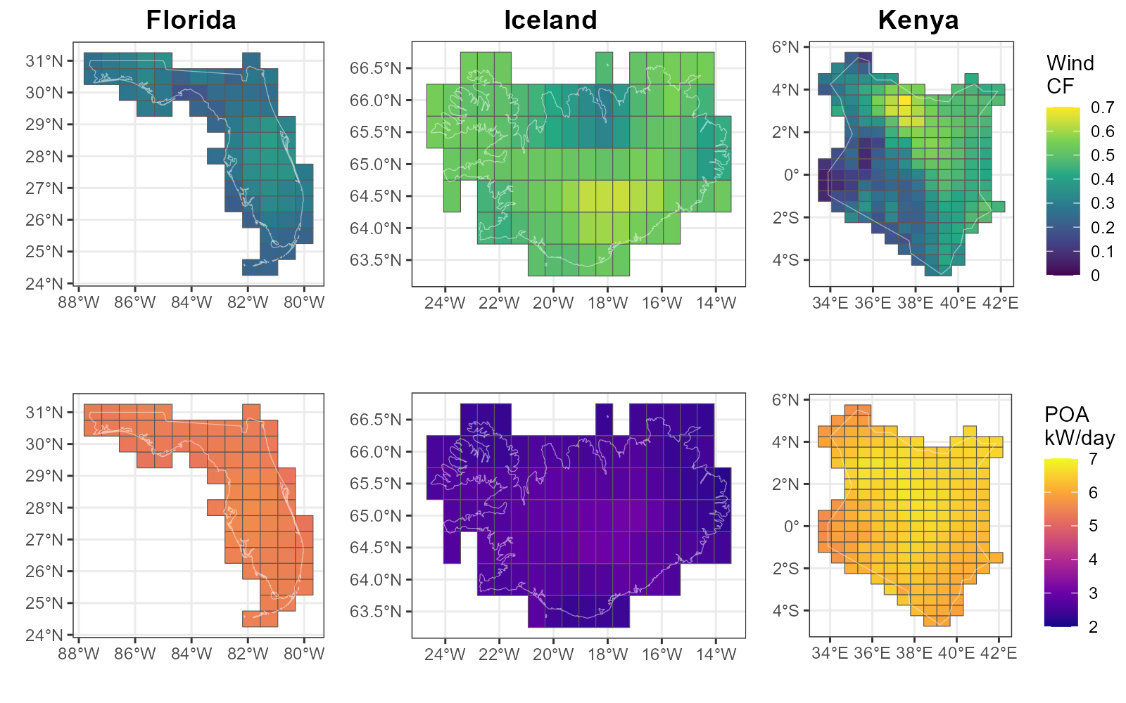
Wind power capacity factors (CF) and Solar irradiance on Plane of Array (POA) by regions
Precipitation by months
prec_ken_m <- merra_ken %>%
  mutate(
    local_time = lubridate::with_tz(UTC, "Africa/Nairobi"),
    year = year(local_time),
    month = month(local_time),
    month_name = factor(month.name[month], levels = month.name, ordered = TRUE)) %>%
  group_by(locid, year, month, month_name) %>%
  summarise(
    PRECTOTCORR = sum(PRECTOTCORR, na.rm = T),
    T10M = mean(T10M),
    .groups = "drop"
    ) %>%
  add_merra2_grid()
code
pre_range <- range(prec_ken_m$PRECTOTCORR)
pre_breaks <- scales::breaks_pretty(5)(pre_range)
pre_range <- range(pre_breaks)
cf_plot(prec_ken_m, kenya_sf, "PRECTOTCORR", brakes = pre_breaks, legend_position = "right") +
facet_wrap(.~month)
ggplot(prec_ken_m) +
geom_sf(aes(fill = PRECTOTCORR)) +
scale_fill_distiller(palette = "YlGnBu", direction = 1, name = "mm /\nmonth") +
facet_wrap(.~month_name) +
geom_sf(data = kenya_sf, fill = NA, colour = alpha("black", .5)) +
theme_bw() + labs(x = "", y = "")
ggsave("images/precipitation_m_kenya.png", scale = 1.5, width = 5, height = 5)
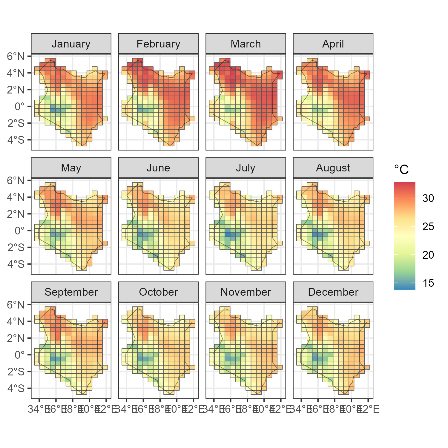
ggplot(prec_ken_m) +
geom_sf(aes(fill = T10M)) +
scale_fill_distiller(palette = "Spectral", direction = -1, name = "\u00B0C") +
facet_wrap(.~month_name) +
geom_sf(data = kenya_sf, fill = NA, colour = alpha("black", .5)) +
theme_bw()
ggsave("images/temperature_m_kenya.png", scale = 1.5, width = 5, height = 5)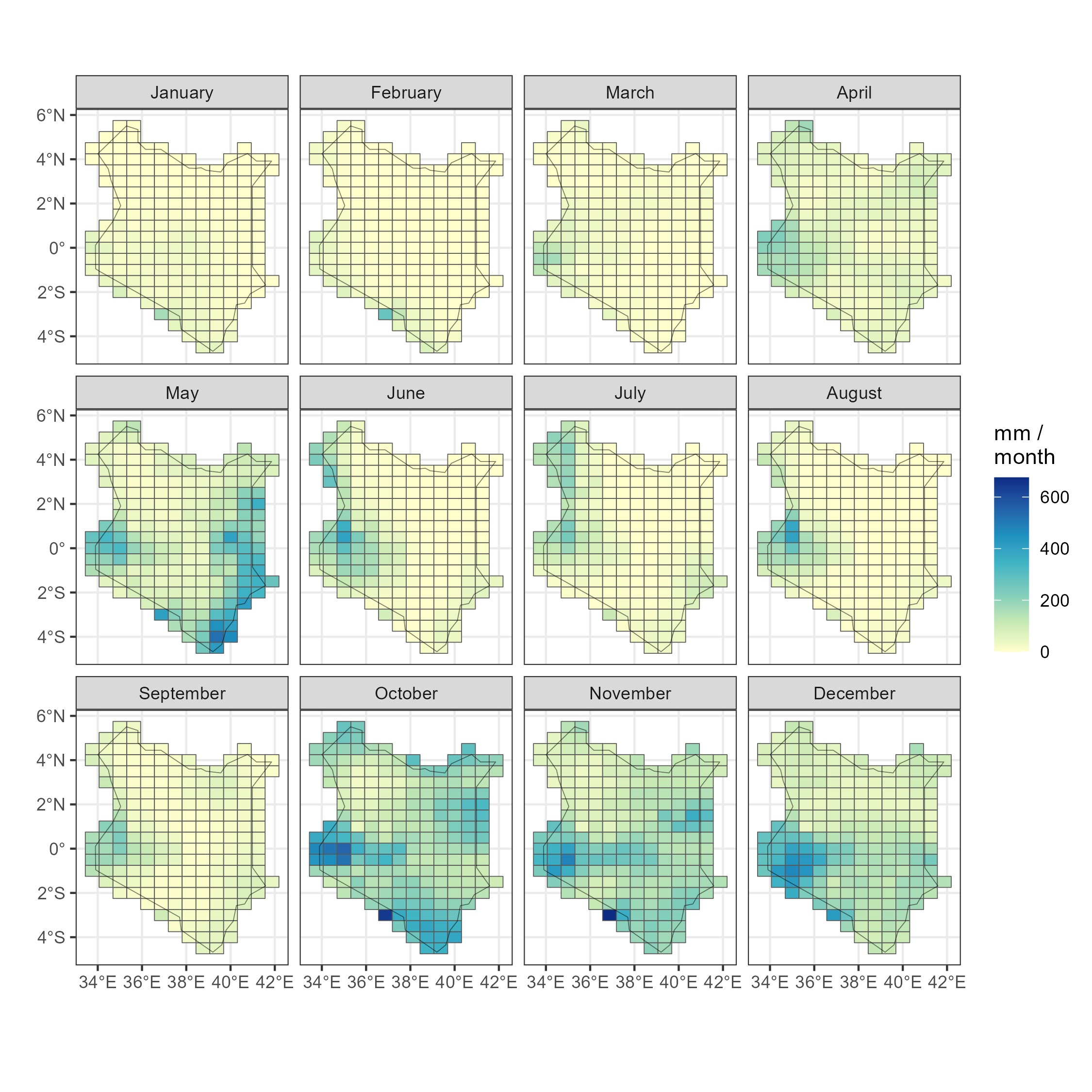
Precipitation by month in Kenya (2019), millimeters / hour (kg/m^2/hour)